Upload Measurement Data and run Analysis#
Now you will post your measurement data and analysis to the database via the API.
If you are running the tutorials in DoLab, the following instructions are not necessary and you can skip directly to the next cell.
You will need to authenticate to the database with your username and password. To make this easy, you can create a file called .env in this folder and complete it with your organization’s URL and authentication information as follows:
dodata_url=https://animal.doplaydo.com
dodata_user=demo
dodata_password=yours
dodata_db=animal.dodata.db.doplaydo.com
dodata_db_user=full_access
dodata_db_password=yours
If you haven’t defined a .env file or saved your credentials to your environment variables, you will be prompted for your credentials now.
import doplaydo.dodata as dd
import pandas as pd
from pathlib import Path
from tqdm.auto import tqdm
import requests
import getpass
from httpx import HTTPStatusError
Let’s now create a project.
In normal circumstances, everyone will be sharing and contributing to a project. In this demo, however, we want to keep your project separate from other users for clarity, so we will append your username to the project name. This way you can also safely delete and recreate projects without creating issues for others. If you prefer though, you can change the PROJECT_ID to anything you like. Just be sure to update it in the subsequent notebooks of this tutorial as well.
username = getpass.getuser()
PROJECT_ID = f"spirals-{username}"
MEASUREMENTS_PATH = Path("6d4c615ff105/")
PROJECT_ID
'spirals-runner'
Lets delete the project if it already exists so that you can start fresh.
try:
    dd.project.delete(project_id=PROJECT_ID).text
except HTTPStatusError:
    pass
New project#
You can create the project, upload the design manifest, and upload the wafer definitions through the Webapp as well as programmatically using this notebook
Upload Project#
You can create a new project and extract all cells & devices below for the RidgeLoss and RibLoss
The expressions are regex expressions. For intro and testing your regexes you can check out regex101
To only extract top cells set max_hierarchy_lvl=-1 and min_hierarchy_lvl=-1
To disable extraction use a max_hierarchy_lvl < min_hierarchy_lvl
Whitelists take precedence over blacklists, so if you define both, it uses only the whitelist.
cell_extraction = [
    dd.project.Extraction(
        cell_id="RibLoss",
        cell_white_list=["^cutback_rib"],
        min_hierarchy_lvl=0,
        max_hierarchy_lvl=0,
    ),
    dd.project.Extraction(
        cell_id="RidgeLoss",
        cell_white_list=["^cutback_ridge"],
        min_hierarchy_lvl=0,
        max_hierarchy_lvl=0,
    ),
]

dd.project.create(
    project_id=PROJECT_ID,
    eda_file="test_chip.gds",
    lyp_file="loss_measurements.lyp",
    cell_extractions=cell_extraction,
).text
'{"success":21}'
Upload Design Manifest#
The design manifest is a CSV file that includes all the cell names, the cell settings, a list of analysis to trigger, and a list of settings for each analysis.
dm = pd.read_csv("design_manifest.csv")
dm
| cell | x | y | width_um | length_um | analysis | analysis_parameters | |
|---|---|---|---|---|---|---|---|
| 0 | cutback_rib_assembled_MFalse_W0p3_L0 | 20150 | 60150 | 0.3 | 0 | [power_envelope] | [{"n": 10, "wvl_of_interest_nm": 1550}] |
| 1 | cutback_rib_assembled_MTrue_W0p3_L25000 | 1039250 | 60150 | 0.3 | 25000 | [power_envelope] | [{"n": 10, "wvl_of_interest_nm": 1550}] |
| 2 | cutback_rib_assembled_MFalse_W0p3_L5000 | 20150 | 204150 | 0.3 | 5000 | [power_envelope] | [{"n": 10, "wvl_of_interest_nm": 1550}] |
| 3 | cutback_rib_assembled_MTrue_W0p3_L20000 | 1039250 | 204150 | 0.3 | 20000 | [power_envelope] | [{"n": 10, "wvl_of_interest_nm": 1550}] |
| 4 | cutback_rib_assembled_MFalse_W0p3_L10000 | 20150 | 348150 | 0.3 | 10000 | [power_envelope] | [{"n": 10, "wvl_of_interest_nm": 1550}] |
| 5 | cutback_rib_assembled_MTrue_W0p3_L15000 | 1039250 | 348150 | 0.3 | 15000 | [power_envelope] | [{"n": 10, "wvl_of_interest_nm": 1550}] |
| 6 | cutback_rib_assembled_MFalse_W0p5_L0 | 20250 | 492250 | 0.5 | 0 | [power_envelope] | [{"n": 10, "wvl_of_interest_nm": 1550}] |
| 7 | cutback_rib_assembled_MTrue_W0p5_L25000 | 1058750 | 492250 | 0.5 | 25000 | [power_envelope] | [{"n": 10, "wvl_of_interest_nm": 1550}] |
| 8 | cutback_rib_assembled_MFalse_W0p5_L5000 | 20250 | 646250 | 0.5 | 5000 | [power_envelope] | [{"n": 10, "wvl_of_interest_nm": 1550}] |
| 9 | cutback_rib_assembled_MTrue_W0p5_L20000 | 1058750 | 646250 | 0.5 | 20000 | [power_envelope] | [{"n": 10, "wvl_of_interest_nm": 1550}] |
| 10 | cutback_rib_assembled_MFalse_W0p5_L10000 | 20250 | 800250 | 0.5 | 10000 | [power_envelope] | [{"n": 10, "wvl_of_interest_nm": 1550}] |
| 11 | cutback_rib_assembled_MTrue_W0p5_L15000 | 1058750 | 800250 | 0.5 | 15000 | [power_envelope] | [{"n": 10, "wvl_of_interest_nm": 1550}] |
| 12 | cutback_rib_assembled_MFalse_W0p8_L0 | 20400 | 954400 | 0.8 | 0 | [power_envelope] | [{"n": 10, "wvl_of_interest_nm": 1550}] |
| 13 | cutback_rib_assembled_MTrue_W0p8_L25000 | 1088000 | 954400 | 0.8 | 25000 | [power_envelope] | [{"n": 10, "wvl_of_interest_nm": 1550}] |
| 14 | cutback_rib_assembled_MFalse_W0p8_L5000 | 20400 | 1123400 | 0.8 | 5000 | [power_envelope] | [{"n": 10, "wvl_of_interest_nm": 1550}] |
| 15 | cutback_rib_assembled_MTrue_W0p8_L20000 | 1088000 | 1123400 | 0.8 | 20000 | [power_envelope] | [{"n": 10, "wvl_of_interest_nm": 1550}] |
| 16 | cutback_rib_assembled_MFalse_W0p8_L10000 | 20400 | 1292400 | 0.8 | 10000 | [power_envelope] | [{"n": 10, "wvl_of_interest_nm": 1550}] |
| 17 | cutback_rib_assembled_MTrue_W0p8_L15000 | 1088000 | 1292400 | 0.8 | 15000 | [power_envelope] | [{"n": 10, "wvl_of_interest_nm": 1550}] |
| 18 | cutback_ridge_assembled_MFalse_W0p3_L0 | 20150 | 60150 | 0.3 | 0 | [power_envelope] | [{"n": 10, "wvl_of_interest_nm": 1550}] |
| 19 | cutback_ridge_assembled_MTrue_W0p3_L25000 | 1037250 | 60150 | 0.3 | 25000 | [power_envelope] | [{"n": 10, "wvl_of_interest_nm": 1550}] |
| 20 | cutback_ridge_assembled_MFalse_W0p3_L5000 | 20150 | 203150 | 0.3 | 5000 | [power_envelope] | [{"n": 10, "wvl_of_interest_nm": 1550}] |
| 21 | cutback_ridge_assembled_MTrue_W0p3_L20000 | 1037250 | 203150 | 0.3 | 20000 | [power_envelope] | [{"n": 10, "wvl_of_interest_nm": 1550}] |
| 22 | cutback_ridge_assembled_MFalse_W0p3_L10000 | 20150 | 346150 | 0.3 | 10000 | [power_envelope] | [{"n": 10, "wvl_of_interest_nm": 1550}] |
| 23 | cutback_ridge_assembled_MTrue_W0p3_L15000 | 1037250 | 346150 | 0.3 | 15000 | [power_envelope] | [{"n": 10, "wvl_of_interest_nm": 1550}] |
| 24 | cutback_ridge_assembled_MFalse_W0p5_L0 | 20250 | 489250 | 0.5 | 0 | [power_envelope] | [{"n": 10, "wvl_of_interest_nm": 1550}] |
| 25 | cutback_ridge_assembled_MTrue_W0p5_L25000 | 1056750 | 489250 | 0.5 | 25000 | [power_envelope] | [{"n": 10, "wvl_of_interest_nm": 1550}] |
| 26 | cutback_ridge_assembled_MFalse_W0p5_L5000 | 20250 | 642250 | 0.5 | 5000 | [power_envelope] | [{"n": 10, "wvl_of_interest_nm": 1550}] |
| 27 | cutback_ridge_assembled_MTrue_W0p5_L20000 | 1056750 | 642250 | 0.5 | 20000 | [power_envelope] | [{"n": 10, "wvl_of_interest_nm": 1550}] |
| 28 | cutback_ridge_assembled_MFalse_W0p5_L10000 | 20250 | 795250 | 0.5 | 10000 | [power_envelope] | [{"n": 10, "wvl_of_interest_nm": 1550}] |
| 29 | cutback_ridge_assembled_MTrue_W0p5_L15000 | 1056750 | 795250 | 0.5 | 15000 | [power_envelope] | [{"n": 10, "wvl_of_interest_nm": 1550}] |
| 30 | cutback_ridge_assembled_MFalse_W0p8_L0 | 20400 | 948400 | 0.8 | 0 | [power_envelope] | [{"n": 10, "wvl_of_interest_nm": 1550}] |
| 31 | cutback_ridge_assembled_MTrue_W0p8_L25000 | 1086000 | 948400 | 0.8 | 25000 | [power_envelope] | [{"n": 10, "wvl_of_interest_nm": 1550}] |
| 32 | cutback_ridge_assembled_MFalse_W0p8_L5000 | 20400 | 1116400 | 0.8 | 5000 | [power_envelope] | [{"n": 10, "wvl_of_interest_nm": 1550}] |
| 33 | cutback_ridge_assembled_MTrue_W0p8_L20000 | 1086000 | 1116400 | 0.8 | 20000 | [power_envelope] | [{"n": 10, "wvl_of_interest_nm": 1550}] |
| 34 | cutback_ridge_assembled_MFalse_W0p8_L10000 | 20400 | 1284400 | 0.8 | 10000 | [power_envelope] | [{"n": 10, "wvl_of_interest_nm": 1550}] |
| 35 | cutback_ridge_assembled_MTrue_W0p8_L15000 | 1086000 | 1284400 | 0.8 | 15000 | [power_envelope] | [{"n": 10, "wvl_of_interest_nm": 1550}] |
dm = dm.drop(columns=["analysis", "analysis_parameters"])
dm
| cell | x | y | width_um | length_um | |
|---|---|---|---|---|---|
| 0 | cutback_rib_assembled_MFalse_W0p3_L0 | 20150 | 60150 | 0.3 | 0 |
| 1 | cutback_rib_assembled_MTrue_W0p3_L25000 | 1039250 | 60150 | 0.3 | 25000 |
| 2 | cutback_rib_assembled_MFalse_W0p3_L5000 | 20150 | 204150 | 0.3 | 5000 |
| 3 | cutback_rib_assembled_MTrue_W0p3_L20000 | 1039250 | 204150 | 0.3 | 20000 |
| 4 | cutback_rib_assembled_MFalse_W0p3_L10000 | 20150 | 348150 | 0.3 | 10000 |
| 5 | cutback_rib_assembled_MTrue_W0p3_L15000 | 1039250 | 348150 | 0.3 | 15000 |
| 6 | cutback_rib_assembled_MFalse_W0p5_L0 | 20250 | 492250 | 0.5 | 0 |
| 7 | cutback_rib_assembled_MTrue_W0p5_L25000 | 1058750 | 492250 | 0.5 | 25000 |
| 8 | cutback_rib_assembled_MFalse_W0p5_L5000 | 20250 | 646250 | 0.5 | 5000 |
| 9 | cutback_rib_assembled_MTrue_W0p5_L20000 | 1058750 | 646250 | 0.5 | 20000 |
| 10 | cutback_rib_assembled_MFalse_W0p5_L10000 | 20250 | 800250 | 0.5 | 10000 |
| 11 | cutback_rib_assembled_MTrue_W0p5_L15000 | 1058750 | 800250 | 0.5 | 15000 |
| 12 | cutback_rib_assembled_MFalse_W0p8_L0 | 20400 | 954400 | 0.8 | 0 |
| 13 | cutback_rib_assembled_MTrue_W0p8_L25000 | 1088000 | 954400 | 0.8 | 25000 |
| 14 | cutback_rib_assembled_MFalse_W0p8_L5000 | 20400 | 1123400 | 0.8 | 5000 |
| 15 | cutback_rib_assembled_MTrue_W0p8_L20000 | 1088000 | 1123400 | 0.8 | 20000 |
| 16 | cutback_rib_assembled_MFalse_W0p8_L10000 | 20400 | 1292400 | 0.8 | 10000 |
| 17 | cutback_rib_assembled_MTrue_W0p8_L15000 | 1088000 | 1292400 | 0.8 | 15000 |
| 18 | cutback_ridge_assembled_MFalse_W0p3_L0 | 20150 | 60150 | 0.3 | 0 |
| 19 | cutback_ridge_assembled_MTrue_W0p3_L25000 | 1037250 | 60150 | 0.3 | 25000 |
| 20 | cutback_ridge_assembled_MFalse_W0p3_L5000 | 20150 | 203150 | 0.3 | 5000 |
| 21 | cutback_ridge_assembled_MTrue_W0p3_L20000 | 1037250 | 203150 | 0.3 | 20000 |
| 22 | cutback_ridge_assembled_MFalse_W0p3_L10000 | 20150 | 346150 | 0.3 | 10000 |
| 23 | cutback_ridge_assembled_MTrue_W0p3_L15000 | 1037250 | 346150 | 0.3 | 15000 |
| 24 | cutback_ridge_assembled_MFalse_W0p5_L0 | 20250 | 489250 | 0.5 | 0 |
| 25 | cutback_ridge_assembled_MTrue_W0p5_L25000 | 1056750 | 489250 | 0.5 | 25000 |
| 26 | cutback_ridge_assembled_MFalse_W0p5_L5000 | 20250 | 642250 | 0.5 | 5000 |
| 27 | cutback_ridge_assembled_MTrue_W0p5_L20000 | 1056750 | 642250 | 0.5 | 20000 |
| 28 | cutback_ridge_assembled_MFalse_W0p5_L10000 | 20250 | 795250 | 0.5 | 10000 |
| 29 | cutback_ridge_assembled_MTrue_W0p5_L15000 | 1056750 | 795250 | 0.5 | 15000 |
| 30 | cutback_ridge_assembled_MFalse_W0p8_L0 | 20400 | 948400 | 0.8 | 0 |
| 31 | cutback_ridge_assembled_MTrue_W0p8_L25000 | 1086000 | 948400 | 0.8 | 25000 |
| 32 | cutback_ridge_assembled_MFalse_W0p8_L5000 | 20400 | 1116400 | 0.8 | 5000 |
| 33 | cutback_ridge_assembled_MTrue_W0p8_L20000 | 1086000 | 1116400 | 0.8 | 20000 |
| 34 | cutback_ridge_assembled_MFalse_W0p8_L10000 | 20400 | 1284400 | 0.8 | 10000 |
| 35 | cutback_ridge_assembled_MTrue_W0p8_L15000 | 1086000 | 1284400 | 0.8 | 15000 |
dm.to_csv("design_manifest_without_analysis.csv", index=False)
dd.project.upload_design_manifest(
    project_id=PROJECT_ID, filepath="design_manifest_without_analysis.csv"
).text
'{"success":200}'
dd.project.download_design_manifest(
    project_id=PROJECT_ID, filepath="design_manifest_downloaded.csv"
)
PosixPath('design_manifest_downloaded.csv')
Upload Wafer Definitions#
The wafer definition is a JSON file where you can define the wafer names and die names and location for each wafer.
dd.project.upload_wafer_definitions(
    project_id=PROJECT_ID, filepath="wafer_definitions.json"
).text
'{"success":200}'
Upload data#
Your Tester can output the data in JSON files. It does not need to be Python.
You can get all paths which have measurement data within the test path.
data_files = list(MEASUREMENTS_PATH.glob("**/data.json"))
print(data_files[0].parts)
('6d4c615ff105', '-2_0', 'RibLoss_cutback_rib_assembled_MFalse_W0p5_L0_20250_492250', 'data.json')
You should define a plotting per measurement type in python. Your plots can evolve over time even for the same measurement type.
Required:
- x_name (str): x-axis name
- y_name (str): y-axis name
- x_col (str): x-column to plot
- y_col (list[str]): y-column(s) to plot; can be multiple
Optional:
- scatter (bool): whether to plot as scatter as opposed to line traces
- x_units (str): x-axis units
- y_units (str): y-axis units
- x_log_axis (bool): whether to plot the x-axis on log scale
- y_log_axis (bool): whether to plot the y-axis on log scale
- x_limits (list[int, int]): clip x-axis data using these limits as bounds (example: [10, 100])
- y_limits (list[int, int]): clip y-axis data using these limits as bounds (example: [20, 100])
- sort_by (dict[str, bool]): columns to sort data before plotting. Boolean specifies whether to sort each column in ascending order.
                             (example: {"wavelegths": True, "optical_power": False})
- grouping (dict[str, int]): columns to group data before plotting. Integer specifies decimal places to round each column.
                             Different series will be plotted for unique combinations of x column, y column(s), and rounded column values.
                             (example: {"port": 1, "attenuation": 2})
spectrum_measurement_type = dd.api.device_data.PlottingKwargs(
    x_name="wavelength",
    y_name="output_power",
    x_col="wavelength",
    y_col=["output_power"],
)
Upload measurements#
You can now upload measurement data.
This is a bare bones example, in a production setting, you can also add validation, logging, and error handling to ensure a smooth operation.
Every measurement you upload will trigger all the analysis that you defined in the design manifest.
NUMBER_OF_THREADS = 1 if "127" in dd.settings.dodata_url else dd.settings.n_threads
NUMBER_OF_THREADS
1
if NUMBER_OF_THREADS == 1:
    for path in tqdm(data_files):
        wafer_id = path.parts[0]
        die_x, die_y = path.parts[1].split("_")

        r = dd.api.device_data.upload(
            file=path,
            project_id=PROJECT_ID,
            wafer_id=wafer_id,
            die_x=die_x,
            die_y=die_y,
            device_id=path.parts[2],
            data_type="measurement",  # can also be "simulation"
            plotting_kwargs=spectrum_measurement_type,
        )
        r.raise_for_status()
data_files = list(MEASUREMENTS_PATH.glob("**/data.json"))
project_ids = []
device_ids = []
die_ids = []
die_xs = []
die_ys = []
wafer_ids = []
plotting_kwargs = []
data_types = []

for path in data_files:
    device_id = path.parts[2]
    die_id = path.parts[1]
    die_x, die_y = die_id.split("_")
    wafer_id = path.parts[0]

    device_ids.append(device_id)
    die_ids.append(die_id)
    die_xs.append(die_x)
    die_ys.append(die_y)
    wafer_ids.append(wafer_id)
    plotting_kwargs.append(spectrum_measurement_type)
    project_ids.append(PROJECT_ID)
    data_types.append("measurement")
if NUMBER_OF_THREADS > 1:
    dd.device_data.upload_multi(
        files=data_files,
        project_ids=project_ids,
        wafer_ids=wafer_ids,
        die_xs=die_xs,
        die_ys=die_ys,
        device_ids=device_ids,
        data_types=data_types,
        plotting_kwargs=plotting_kwargs,
        progress_bar=True,
    )
wafer_set = set(wafer_ids)
die_set = set(die_ids)

print(wafer_set)
print(die_set)
print(len(die_set))
{'6d4c615ff105'}
{'2_1', '-1_0', '-1_-1', '0_2', '2_-1', '0_-1', '-1_2', '1_1', '-2_0', '0_0', '1_-2', '0_-2', '-2_1', '1_2', '-2_-1', '-1_-2', '1_0', '1_-1', '0_1', '-1_1', '2_0'}
21
Analysis#
You can run analysis at 3 different levels. For example to calculate:
Device: averaged power envelope over certain number of samples.
Die: fit the propagation loss as a function of length.
Wafer: Define the Upper and Lower Spec limits for Known Good Die (KGD)

To upload custom analysis functions to the DoData server, follow these simplified guidelines:
Input:
Begin with a unique identifier (device_data_id, die_id, wafer_id) as the first argument.
Add necessary keyword arguments for the analysis.
Output: Dictionary
output: Return a simple, one-level dictionary. All values must be serializable. Avoid using numpy or pandas; convert to lists if needed.
summary_plot: Provide a summary plot, either as a matplotlib figure or io.BytesIO object.
attributes: Add a serializable dictionary of the analysis settings.
device_data_id/die_id/wafer_id: Include the used identifier (device_data_id, die_id, wafer_id).
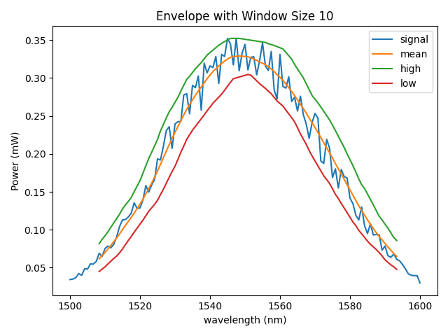
Device Analysis#
You can either trigger analysis automatically by defining it in the design manifest, using the UI or using the Python DoData library.
from IPython.display import Code, display, Image
import doplaydo.dodata as dd

display(Code(dd.config.Path.analysis_functions_device_power_envelope))
"""This module contains the power_envelope function."""

from typing import Any
import numpy as np
from matplotlib import pyplot as plt
import doplaydo.dodata as dd


def run(
    device_data_pkey: int,
    n: int = 500,
    wvl_of_interest_nm: float = 1550,
    xkey: str = "wavelength",
    ykey: str = "output_power",
    convert_to_dB: bool = False,
) -> dict[str, Any]:
    """Returns the smoothen data using a window averaging of a 1d array.

    Args:
        device_data_pkey: device data pkey.
        n: points per window.
        wvl_of_interest_nm: wavelength of interest.
        xkey: xkey.
        ykey: ykey.
        convert_to_dB: if True, convert power to dB.
    """
    data = dd.get_data_by_pkey(device_data_pkey)

    if data is None:
        raise ValueError(f"Device data with pkey {device_data_pkey} not found.")

    if xkey not in data:
        raise ValueError(
            f"Device data with pkey {device_data_pkey} does not have xkey {xkey!r}."
        )

    if ykey not in data:
        raise ValueError(
            f"Device data with pkey {device_data_pkey} does not have ykey {ykey!r}."
        )

    wavelength = data[xkey].values
    power = data[ykey].values
    power = 10 * np.log10(power) if convert_to_dB else power

    closest_wvl_index = np.argmin(np.abs(wavelength - wvl_of_interest_nm))

    mean_curve = (
        data.output_power.rolling(n, center=True).mean().rolling(n, center=True).mean()
    )
    low_curve = (
        data.output_power.rolling(n, center=True).min().rolling(n, center=True).mean()
    )
    high_curve = (
        data.output_power.rolling(n, center=True).max().rolling(n, center=True).mean()
    )

    fig = plt.figure()
    plt.plot(wavelength, power, label="signal", zorder=0)
    plt.plot(wavelength, mean_curve, label="mean", zorder=1)
    plt.plot(wavelength, high_curve, label="high", zorder=1)
    plt.plot(wavelength, low_curve, label="low", zorder=1)

    ylabel = "Power (dBm)" if convert_to_dB else "Power (mW)"
    plt.xlabel("wavelength (nm)")
    plt.ylabel(ylabel)
    plt.legend()
    plt.title(f"Envelope with Window Size {n}")
    plt.close()

    return dict(
        output={
            "closest_wavelength_value_nm": float(wavelength[closest_wvl_index]),
            "mean_wavelength_value_nm": float(mean_curve[closest_wvl_index]),
            "low_wavelength_value_nm": float(low_curve[closest_wvl_index]),
            "high_wavelength_value_nm": float(high_curve[closest_wvl_index]),
        },
        summary_plot=fig,
        device_data_pkey=device_data_pkey,
    )


if __name__ == "__main__":
    d = run(77404)
    print(d["output"]["closest_wavelength_value_nm"])
device_data, df = dd.get_data_by_query([dd.Project.project_id == PROJECT_ID], limit=1)[
    0
]
device_data.pkey
7215
analysis_function_id = "device_power_envelope"

response = dd.api.analysis_functions.validate(
    analysis_function_id=analysis_function_id,
    function_path=dd.config.Path.analysis_functions_device_power_envelope,
    test_model_pkey=device_data.pkey,
    target_model_name="device_data",
    parameters=dict(n=10),
)
Image(response.content)
Headers({'server': 'nginx/1.22.1', 'date': 'Fri, 28 Feb 2025 21:05:09 GMT', 'content-type': 'image/png', 'transfer-encoding': 'chunked', 'connection': 'keep-alive', '_output': '{"closest_wavelength_value_nm": 1550.0, "mean_wavelength_value_nm": 0.32842423409232385, "low_wavelength_value_nm": 0.3035408903939654, "high_wavelength_value_nm": 0.35102408190763246}', '_attributes': '{}', '_device_data_pkey': '7215', 'strict-transport-security': 'max-age=63072000'})
analysis_function_id = "device_power_envelope"

dd.api.analysis_functions.validate_and_upload(
    analysis_function_id=analysis_function_id,
    function_path=dd.config.Path.analysis_functions_device_power_envelope,
    test_model_pkey=device_data.pkey,
    target_model_name="device_data",
)
Headers({'server': 'nginx/1.22.1', 'date': 'Fri, 28 Feb 2025 21:05:10 GMT', 'content-type': 'image/png', 'transfer-encoding': 'chunked', 'connection': 'keep-alive', '_output': '{"closest_wavelength_value_nm": 1550.0, "mean_wavelength_value_nm": null, "low_wavelength_value_nm": null, "high_wavelength_value_nm": null}', '_attributes': '{}', '_device_data_pkey': '7215', 'strict-transport-security': 'max-age=63072000'})
<Response [200 OK]>
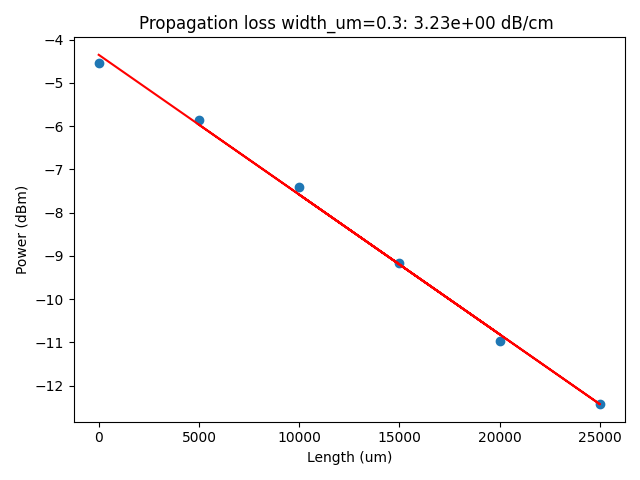
Die Analysis#
You can trigger a die analysis for 300, 500 and 800nm wide waveguides.
Code(dd.config.Path.analysis_functions_die_loss_cutback)
"""Calculates propagation loss from cutback measurement."""

from typing import Any
import numpy as np
from matplotlib import pyplot as plt

import doplaydo.dodata as dd


def run(
    die_pkey: int,
    key: str = "width_um",
    value: float = 0.3,
    length_key: str = "length_um",
    convert_to_dB: bool = True,
) -> dict[str, Any]:
    """Returns propagation loss in dB/cm.

    Args:
        die_pkey: pkey of the die to analyze.
        key: key of the attribute to filter by.
        value: value of the attribute to filter by.
        length_key: key of the length attribute.
        convert_to_dB: if True, convert power to dB.
    """
    device_data_objects = dd.get_data_by_query(
        [dd.Die.pkey == die_pkey, dd.attribute_filter(dd.Cell, key, value)]
    )

    if not device_data_objects:
        raise ValueError(
            f"No device data found with die_pkey {die_pkey}, key {key!r}, value {value}"
        )

    powers = []
    lengths_um = []

    for device_data, df in device_data_objects:
        lengths_um.append(device_data.device.cell.attributes.get(length_key))
        power = df.output_power.max()
        power = 10 * np.log10(power) if convert_to_dB else power
        powers.append(power)

    p = np.polyfit(lengths_um, powers, 1)
    propagation_loss = p[0] * 1e4 * -1

    fig = plt.figure()
    plt.plot(lengths_um, powers, "o")
    plt.plot(lengths_um, np.polyval(p, lengths_um), "r-", label="fit")

    ylabel = "Power (dBm)" if convert_to_dB else "Power (mW)"
    plt.xlabel("Length (um)")
    plt.ylabel(ylabel)
    plt.title(f"Propagation loss {key}={value}: {p[0]*1e4*-1:.2e} dB/cm ")

    return dict(
        output={"propagation_loss_dB_cm": propagation_loss},
        summary_plot=fig,
        die_pkey=die_pkey,
    )


if __name__ == "__main__":
    d = run(7732)
    print(d["output"]["propagation_loss_dB_cm"])
Lets find a die pkey for this project, so that we can trigger the die analysis on it.
device_data, df = dd.get_data_by_query([dd.Project.project_id == PROJECT_ID], limit=1)[
    0
]
device_data.die.pkey
795
die_pkey = device_data.die.pkey
response = dd.api.analysis_functions.validate(
    analysis_function_id="die_loss_cutback",
    function_path=dd.config.Path.analysis_functions_die_loss_cutback,
    test_model_pkey=die_pkey,
    target_model_name="die",
)
Image(response.content)
Headers({'server': 'nginx/1.22.1', 'date': 'Fri, 28 Feb 2025 21:05:11 GMT', 'content-type': 'image/png', 'transfer-encoding': 'chunked', 'connection': 'keep-alive', '_output': '{"propagation_loss_dB_cm": 3.232782941876761}', '_attributes': '{}', '_die_pkey': '795', 'strict-transport-security': 'max-age=63072000'})
dd.api.analysis_functions.validate_and_upload(
    analysis_function_id="die_loss_cutback",
    function_path=dd.config.Path.analysis_functions_die_loss_cutback,
    test_model_pkey=die_pkey,
    target_model_name="die",
)
Headers({'server': 'nginx/1.22.1', 'date': 'Fri, 28 Feb 2025 21:05:11 GMT', 'content-type': 'image/png', 'transfer-encoding': 'chunked', 'connection': 'keep-alive', '_output': '{"propagation_loss_dB_cm": 3.232782941876761}', '_attributes': '{}', '_die_pkey': '795', 'strict-transport-security': 'max-age=63072000'})
<Response [200 OK]>
database_dies = []
widths_um = [0.3, 0.5, 0.8]
NUMBER_OF_THREADS = dd.settings.n_threads
widths_um = [0.3, 0.5, 0.8]
parameters = [{"value": width_um, "key": "width_um"} for width_um in widths_um]

dd.analysis.trigger_die_multi(
    project_id=PROJECT_ID,
    analysis_function_id="die_loss_cutback",
    wafer_ids=wafer_set,
    die_xs=die_xs,
    die_ys=die_ys,
    parameters=parameters,
    progress_bar=True,
    n_threads=2,
)
plots = dd.analysis.get_die_analysis_plots(
    project_id=PROJECT_ID, wafer_id=wafer_ids[0], die_x=0, die_y=0
)
len(plots)
3
display(plots[0])
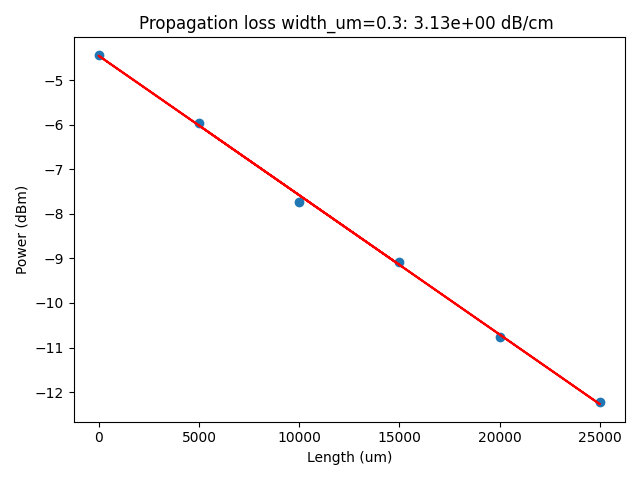
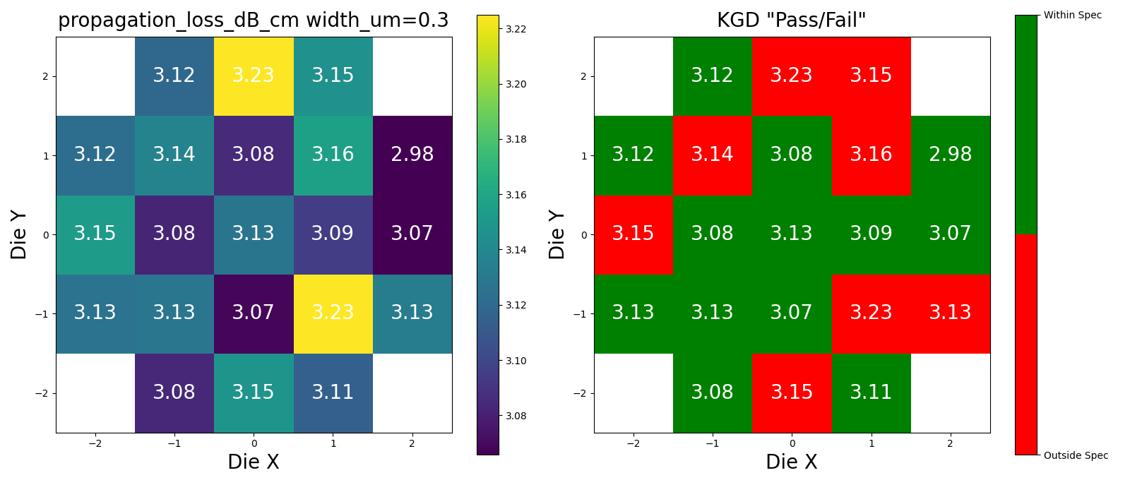
Wafer Analysis#
Lets Define the Upper and Lower Spec limits for Known Good Die (KGD).
For example:
waveguide width (nm) |
Lower Spec Limit (dB/cm) |
Upper Spec limit (dB/cm) |
|---|---|---|
300 |
0 |
3.13 |
500 |
0 |
2.31 |
800 |
0 |
1.09 |
As for waveguide loss you can define no minimum loss (0 dB/cm) and you only define the maximum accepted loss (Upper Spec Limit)
Code(dd.config.Path.analysis_functions_wafer_loss_cutback)
"""Aggregate analysis."""

from typing import Any
import matplotlib.colors as mcolors
import numpy as np
from matplotlib import pyplot as plt
from matplotlib.figure import Figure
from collections import defaultdict

import doplaydo.dodata as dd


def format_float(value: float, decimal_places: int) -> str:
    """Format a float to a string with a fixed number of decimal places.

    Args:
        value: Value to format.
        decimal_places: Number of decimal places to display.
    """
    return f"{value:.{decimal_places}f}"


def plot_wafermap(
    losses: dict[tuple[int, int], float],
    lower_spec: float,
    upper_spec: float,
    metric: str,
    key: str | None = None,
    value: float | None = None,
    decimal_places: int = 2,
    scientific_notation: bool = False,
    fontsize: int = 20,
    fontsize_die: int = 20,
    percentile_low: int = 5,
    percentile_high: int = 95,
) -> Figure:
    """Plot a wafermap of the losses.

    Args:
        losses: Dictionary of losses.
        lower_spec: Lower specification limit.
        upper_spec: Upper specification limit.
        metric: Metric to analyze.
        key: Key of the parameter to analyze.
        value: Value of the parameter to analyze.
        decimal_places: Number of decimal places to display.
        scientific_notation: Whether to display the values in scientific notation.
        fontsize: Font size for the labels.
        fontsize_die: Font size for the die labels.
        percentile_low: Lower percentile for the color scale.
        percentile_high: Upper percentile for the color scale.
    """
    # Calculate the bounds and center of the data
    die_xs, die_ys = zip(*losses.keys())
    die_x_min, die_x_max = min(die_xs), max(die_xs)
    die_y_min, die_y_max = min(die_ys), max(die_ys)

    # Create the data array
    data = np.full((die_y_max - die_y_min + 1, die_x_max - die_x_min + 1), np.nan)
    for (i, j), v in losses.items():
        data[j - die_y_min, i - die_x_min] = v

    fig, (ax1, ax2) = plt.subplots(1, 2, figsize=(16, 6.8))

    # First subplot: Heatmap
    ax1.set_xlabel("Die X", fontsize=fontsize)
    ax1.set_ylabel("Die Y", fontsize=fontsize)
    title = f"{metric} {key}={value}" if value and key else f"{metric}"
    ax1.set_title(title, fontsize=fontsize, pad=10)

    cmap = plt.get_cmap("viridis")
    vmin = np.nanpercentile(list(losses.values()), percentile_low)
    vmax = np.nanpercentile(list(losses.values()), percentile_high)

    heatmap = ax1.imshow(
        data,
        cmap=cmap,
        extent=[die_x_min - 0.5, die_x_max + 0.5, die_y_min - 0.5, die_y_max + 0.5],
        origin="lower",
        vmin=vmin,
        vmax=vmax,
    )

    ax1.set_xlim(die_x_min - 0.5, die_x_max + 0.5)
    ax1.set_ylim(die_y_min - 0.5, die_y_max + 0.5)

    for (i, j), v in losses.items():
        if not np.isnan(v):
            if v is not None:
                value_str = (
                    f"{v:.{decimal_places}e}"
                    if scientific_notation
                    else f"{v:.{decimal_places}f}"
                )
            else:
                value_str = str(v)
            ax1.text(
                i,
                j,
                value_str,
                ha="center",
                va="center",
                color="white",
                fontsize=fontsize_die,
            )

    plt.colorbar(heatmap, ax=ax1)

    # Second subplot: Binary map based on specifications
    binary_map = np.where(
        np.isnan(data),
        np.nan,
        np.where((data >= lower_spec) & (data <= upper_spec), 1, 0),
    )

    cmap_binary = mcolors.ListedColormap(["red", "green"])
    heatmap_binary = ax2.imshow(
        binary_map,
        cmap=cmap_binary,
        extent=[die_x_min - 0.5, die_x_max + 0.5, die_y_min - 0.5, die_y_max + 0.5],
        origin="lower",
        vmin=0,
        vmax=1,
    )

    ax2.set_xlim(die_x_min - 0.5, die_x_max + 0.5)
    ax2.set_ylim(die_y_min - 0.5, die_y_max + 0.5)

    for (i, j), v in losses.items():
        if not np.isnan(v):
            if v is not None:
                value_str = (
                    f"{v:.{decimal_places}e}"
                    if scientific_notation
                    else f"{v:.{decimal_places}f}"
                )
            else:
                value_str = str(v)
            ax2.text(
                i,
                j,
                value_str,
                ha="center",
                va="center",
                color="white",
                fontsize=fontsize_die,
            )

    ax2.set_xlabel("Die X", fontsize=fontsize)
    ax2.set_ylabel("Die Y", fontsize=fontsize)
    ax2.set_title('KGD "Pass/Fail"', fontsize=fontsize, pad=10)
    plt.colorbar(heatmap_binary, ax=ax2, ticks=[0, 1]).set_ticklabels(
        ["Outside Spec", "Within Spec"]
    )
    return fig


def run(
    wafer_pkey: int,
    lower_spec: float,
    upper_spec: float,
    analysis_function_id: str,
    metric: str,
    key: str | None = None,
    value: float | None = None,
    decimal_places: int = 2,
    scientific_notation: bool = False,
    fontsize: int = 20,
    fontsize_die: int = 20,
    percentile_low: int = 5,
    percentile_high: int = 95,
) -> dict[str, Any]:
    """Returns wafer map of metric after analysis_function_id.

    Args:
        wafer_pkey: pkey of the wafer to analyze.
        lower_spec: Lower specification limit.
        upper_spec: Upper specification limit.
        analysis_function_id: Name of the die function to analyze.
        metric: Metric to analyze.
        key: Key of the parameter to analyze.
        value: Value of the parameter to analyze.
        decimal_places: Number of decimal places to display.
        scientific_notation: Whether to display the values in scientific notation.
        fontsize: Font size for the labels.
        fontsize_die: Font size for the die labels.
        percentile_low: Lower percentile for the color scale.
        percentile_high: Upper percentile for the color scale.
    """
    filter_clauses = [dd.AnalysisFunction.analysis_function_id == analysis_function_id]

    if key is not None:
        filter_clauses.append(
            dd.analysis_filter(column_name="parameters", key="key", value=key)
        )
    if value is not None:
        filter_clauses.append(
            dd.analysis_filter(column_name="parameters", key="value", value=value)
        )

    analyses = dd.db.analysis.get_analyses_for_wafer_by_pkey(
        wafer_pkey=wafer_pkey,
        target_model="die",
        filter_clauses=filter_clauses,
    )

    analyses_per_die: dict[tuple[int, int], list[dd.Analysis]] = defaultdict(list)

    for analysis in analyses:
        analyses_per_die[(analysis.die.x, analysis.die.y)].append(analysis)

    result: dict[tuple[int, int], dd.Analysis] = {}
    for coord, analyses in analyses_per_die.items():
        max_analysis_index = np.argmax([a.pkey for a in analyses])
        last_analysis = analyses[max_analysis_index]
        o = last_analysis.output[metric]  # get the last analysis (most recent)
        if not isinstance(o, float | int):
            raise ValueError(f"Analysis output {o} is not a float or int")
        result[coord] = o

    result_list = [value for value in result.values() if isinstance(value, int | float)]
    result_array = np.array(result_list)
    if np.any(np.isnan(result_array)) or not result:
        raise ValueError(
            f"No analysis for {wafer_pkey=} {analysis_function_id=} found."
        )

    summary_plot = plot_wafermap(
        result,
        value=value,
        key=key,
        lower_spec=lower_spec,
        upper_spec=upper_spec,
        metric=metric,
        decimal_places=decimal_places,
        scientific_notation=scientific_notation,
        fontsize=fontsize,
        fontsize_die=fontsize_die,
        percentile_low=percentile_low,
        percentile_high=percentile_high,
    )

    return dict(
        output={"losses": result_list},
        summary_plot=summary_plot,
        wafer_pkey=wafer_pkey,
    )


if __name__ == "__main__":
    parameters = {
        "key": "components",
        "upper_spec": 1.15,
        "lower_spec": 0,
        "analysis_function_id": "die_cutback",
        "metric": "component_loss",
    }
    wafer_pkey = 25
    d = run(wafer_pkey, **parameters)
    print(d["output"]["losses"])
Lets find a wafer pkey for this project, so that we can trigger the wafer analysis on it.
device_data, df = dd.get_data_by_query([dd.Project.project_id == PROJECT_ID], limit=1)[
    0
]
wafer_pkey = device_data.die.wafer.pkey
wafer_pkey
26
response = dd.api.analysis_functions.validate(
    analysis_function_id="wafer_loss_cutback",
    function_path=dd.config.Path.analysis_functions_wafer_loss_cutback,
    test_model_pkey=wafer_pkey,
    target_model_name="wafer",
    parameters={
        "key": "width_um",
        "value": 0.3,
        "upper_spec": 3.13,
        "lower_spec": 0,
        "analysis_function_id": "die_loss_cutback",
        "metric": "propagation_loss_dB_cm",
    },
)
Image(response.content)
Headers({'server': 'nginx/1.22.1', 'date': 'Fri, 28 Feb 2025 21:05:31 GMT', 'content-type': 'image/png', 'transfer-encoding': 'chunked', 'connection': 'keep-alive', '_output': '{"losses": [3.128042413979003, 3.1147472028889727, 3.14814962163856, 3.146460405000149, 3.232782941876761, 3.084309519793603, 3.1563920593037, 3.0847608622286886, 3.09441691155175, 3.1194603708110686, 2.975176653200896, 3.127712573325798, 3.0657491399999373, 3.123311215374098, 3.2250855372322693, 3.152948408222198, 3.0682798055598965, 3.1325809673774585, 3.1370797291024304, 3.12647883013988, 3.0821871764516517]}', '_attributes': '{}', '_wafer_pkey': '26', 'strict-transport-security': 'max-age=63072000'})

dd.api.analysis_functions.validate_and_upload(
    analysis_function_id="wafer_loss_cutback",
    function_path=dd.config.Path.analysis_functions_wafer_loss_cutback,
    test_model_pkey=wafer_pkey,
    target_model_name="wafer",
    parameters={
        "key": "width_um",
        "value": 0.3,
        "lower_spec": 0,
        "upper_spec": 3.13,
        "analysis_function_id": "die_loss_cutback",
        "metric": "propagation_loss_dB_cm",
    },
)
Headers({'server': 'nginx/1.22.1', 'date': 'Fri, 28 Feb 2025 21:05:32 GMT', 'content-type': 'image/png', 'transfer-encoding': 'chunked', 'connection': 'keep-alive', '_output': '{"losses": [3.128042413979003, 3.1147472028889727, 3.14814962163856, 3.146460405000149, 3.232782941876761, 3.084309519793603, 3.1563920593037, 3.0847608622286886, 3.09441691155175, 3.1194603708110686, 2.975176653200896, 3.127712573325798, 3.0657491399999373, 3.123311215374098, 3.2250855372322693, 3.152948408222198, 3.0682798055598965, 3.1325809673774585, 3.1370797291024304, 3.12647883013988, 3.0821871764516517]}', '_attributes': '{}', '_wafer_pkey': '26', 'strict-transport-security': 'max-age=63072000'})
<Response [200 OK]>
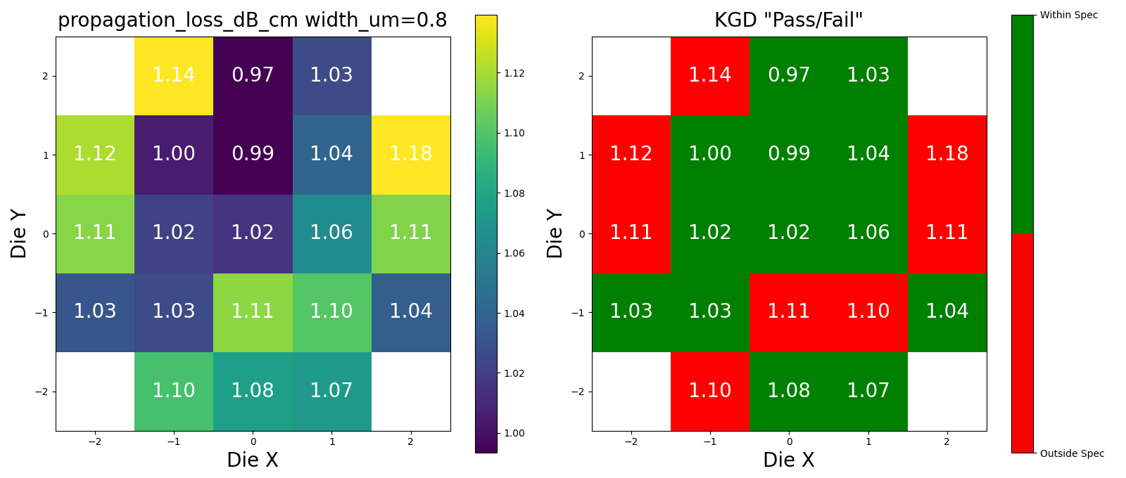
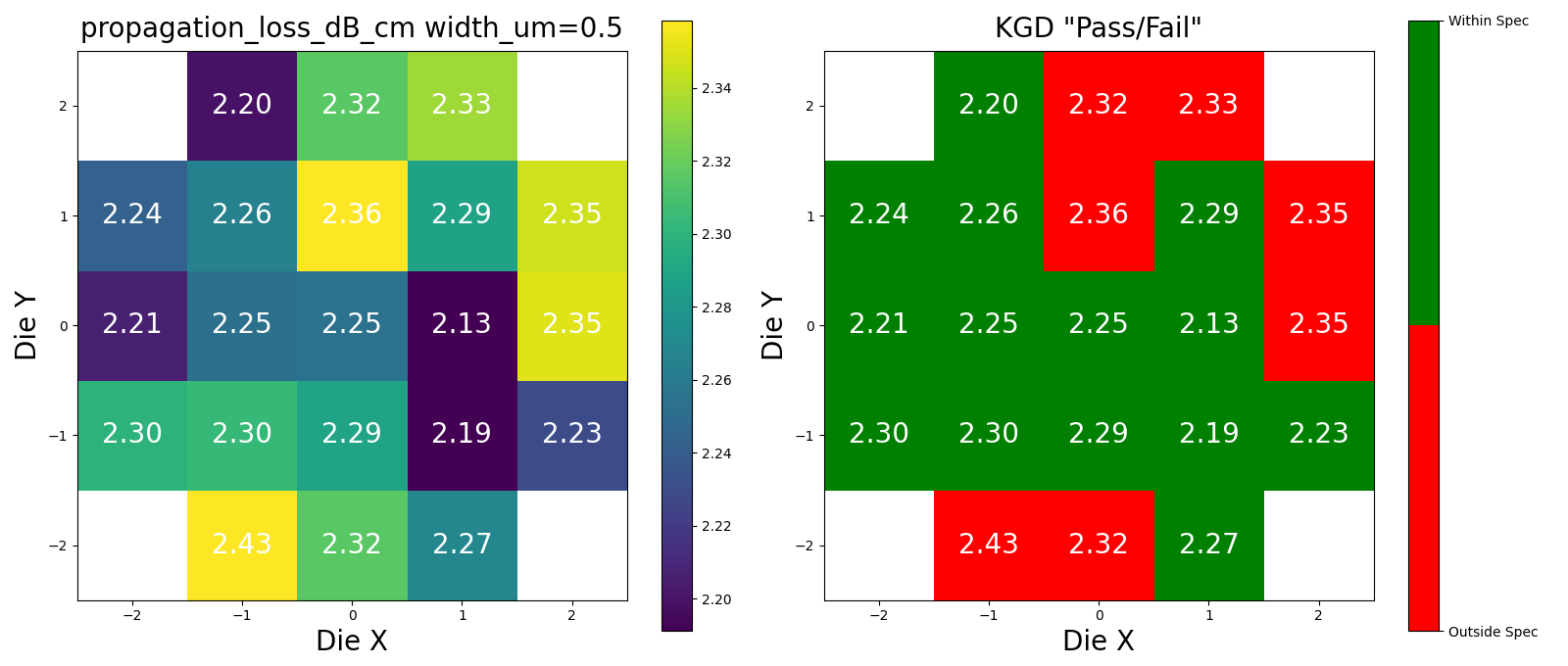
widths_um = [0.3, 0.5, 0.8]
maximum_loss_per_width = {
    0.3: 3.13,
    0.5: 2.31,
    0.8: 1.09,
}
parameters = [
    {
        "key": "width_um",
        "value": width_um,
        "upper_spec": maximum_loss_per_width[width_um],
        "lower_spec": 0,
        "analysis_function_id": "die_loss_cutback",
        "metric": "propagation_loss_dB_cm",
    }
    for width_um in widths_um
]

for wafer in tqdm(wafer_set):
    for params in parameters:
        r = dd.analysis.trigger_wafer(
            project_id=PROJECT_ID,
            wafer_id=wafer,
            analysis_function_id="wafer_loss_cutback",
            parameters=params,
        )
        if r.status_code != 200:
            raise requests.HTTPError(r.text)
plots = dd.analysis.get_wafer_analysis_plots(
    project_id=PROJECT_ID, wafer_id=wafer_ids[0], target_model="wafer"
)
len(plots)
3
for plot in plots:
    display(plot)