Measurements

In this tutorial you will generate some sample (fake) measurement data so you can post it to your project.

You can create a new folder and populate it with JSON files containing the fake measurement data for the whole wafer.

import json
import pandas as pd
import numpy as np
from pathlib import Path
import matplotlib.pyplot as plt

df = pd.read_csv("design_manifest.csv")
df

	cell	x	y	radius_um	gap_um	analysis	analysis_parameters
0	RingDouble-20-0.25-	331580	121311	20	0.25	[fsr]	[{"height": -0.01, "distance": 20}]
1	RingDouble-20-0.2-	331580	285371	20	0.20	[fsr]	[{"height": -0.01, "distance": 20}]
2	RingDouble-20-0.15-	331580	449331	20	0.15	[fsr]	[{"height": -0.01, "distance": 20}]
3	RingDouble-10-0.2-	331480	613191	10	0.20	[fsr]	[{"height": -0.01, "distance": 20}]
4	RingDouble-10-0.15-	331480	757151	10	0.15	[fsr]	[{"height": -0.01, "distance": 20}]
5	RingDouble-10-0.1-	331480	901011	10	0.10	[fsr]	[{"height": -0.01, "distance": 20}]
6	RingDouble-5-0.2-	331480	1044771	5	0.20	[fsr]	[{"height": -0.01, "distance": 20}]
7	RingDouble-5-0.15-	331480	1178731	5	0.15	[fsr]	[{"height": -0.01, "distance": 20}]
8	RingDouble-5-0.1-	331480	1312591	5	0.10	[fsr]	[{"height": -0.01, "distance": 20}]

def ring(
    wl: np.ndarray,
    wl0: float,
    neff: float,
    ng: float,
    ring_length: float,
    coupling: float,
    loss: float,
) -> np.ndarray:
    """Returns Frequency Domain Response of an all pass filter.

    Args:
        wl: wavelength in  um.
        wl0: center wavelength at which neff and ng are defined.
        neff: effective index.
        ng: group index.
        ring_length: in um.
        loss: dB/um.
    """
    transmission = 1 - coupling
    neff_wl = (
        neff + (wl0 - wl) * (ng - neff) / wl0
    )  # we expect a linear behavior with respect to wavelength
    out = np.sqrt(transmission) - 10 ** (-loss * ring_length * 1e-6 / 20.0) * np.exp(
        2j * np.pi * neff_wl * ring_length / wl
    )
    out /= 1 - np.sqrt(transmission) * 10 ** (
        -loss * ring_length * 1e-6 / 20.0
    ) * np.exp(2j * np.pi * neff_wl * ring_length / wl)
    return abs(out) ** 2


def gaussian_grating_coupler_response(
    peak_power, center_wavelength, bandwidth_1dB, wavelength
):
    """Calculate the response of a Gaussian grating coupler.

    Args:
        peak_power: The peak power of the response.
        center_wavelength: The center wavelength of the grating coupler.
        bandwidth_1dB: The 1 dB bandwidth of the coupler.
        wavelength: The wavelength at which the response is evaluated.

    Returns:
        The power of the grating coupler response at the given wavelength.
    """
    # Convert 1 dB bandwidth to standard deviation (sigma)
    sigma = bandwidth_1dB / (2 * np.sqrt(2 * np.log(10)))

    # Gaussian response calculation
    response = peak_power * np.exp(
        -0.5 * ((wavelength - center_wavelength) / sigma) ** 2
    )

    return response


nm = 1e-3
# Parameters
peak_power = 1.0
center_wavelength = 1550 * nm  # Center wavelength in micrometers
bandwidth_1dB = 100 * nm

# Wavelength range: 100 nm around the center wavelength, converted to micrometers
wavelength_range = np.linspace(center_wavelength - 0.05, center_wavelength + 0.05, 500)

# Calculate the response for each wavelength
grating_spectrum = np.array(
    [
        gaussian_grating_coupler_response(
            peak_power, center_wavelength, bandwidth_1dB, wl
        )
        for wl in wavelength_range
    ]
)
ring_spectrum = ring(
    wavelength_range,
    wl0=1.55,
    neff=2.4,
    ng=4.0,
    ring_length=2 * np.pi * 10,
    coupling=0.1,
    loss=30e2,  # 30 dB/cm = 30000 dB/m
)
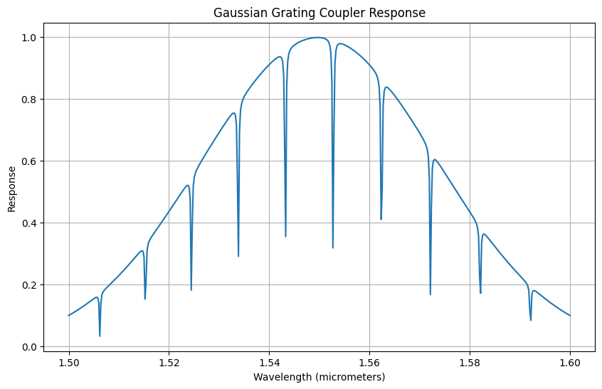
spectrum = ring_spectrum * grating_spectrum

# Plotting
plt.figure(figsize=(10, 6))
plt.plot(wavelength_range, spectrum)
plt.title("Gaussian Grating Coupler Response")
plt.xlabel("Wavelength (micrometers)")
plt.ylabel("Response")
plt.grid(True)
plt.show()

for radius in [5, 10, 20]:
    dB = 3 * (radius * 1e-4 * 2 * 3.14)
    print(10 ** (-dB / 10))

0.9978333154992974
0.9956713255203204
0.9913613884633918

import numpy as np
from scipy.signal import find_peaks


def find_resonance_peaks(
    y, height: float = 0.1, threshold: None | float = None, distance: float | None = 10
):
    """Find the resonance peaks in the ring resonator response.

    'height' and 'distance' can be adjusted based on the specifics of your data.

    Args:
        y: ndarray
        height : number or ndarray or sequence, optional
            Required height of peaks. Either a number, ``None``, an array matching
            `x` or a 2-element sequence of the former. The first element is
            always interpreted as the  minimal and the second, if supplied, as the
            maximal required height.
        threshold : number or ndarray or sequence, optional
            Required threshold of peaks, the vertical distance to its neighboring
            samples. Either a number, ``None``, an array matching `x` or a
            2-element sequence of the former. The first element is always
            interpreted as the  minimal and the second, if supplied, as the maximal
            required threshold.
        distance : number, optional
            Required minimal horizontal distance (>= 1) in samples between
            neighbouring peaks. Smaller peaks are removed first until the condition
            is fulfilled for all remaining peaks.
    """
    if height < 0:
        y = -y
        height = abs(height)

    peaks, _ = find_peaks(y, height=height, distance=distance)
    return peaks


def calculate_FSR(x, peaks):
    """Calculate the Free Spectral Range (FSR) based on the found peaks."""
    peak_frequencies = x[peaks]
    fsr = np.diff(peak_frequencies)
    return fsr


def remove_baseline(wavelength: np.ndarray, power: np.ndarray, deg: int = 4):
    """Return power corrected without baseline.

    Fit a polynomial ``p(x) = p[0] * x**deg + ... + p[deg]`` of degree `deg`
    """
    pfit = np.polyfit(wavelength - np.mean(wavelength), power, deg)
    power_baseline = np.polyval(pfit, wavelength - np.mean(wavelength))

    power_corrected = power - power_baseline
    power_corrected = power_corrected + max(power_baseline) - max(power)
    return power_corrected


x = wavelength_range
y = remove_baseline(wavelength=wavelength_range, power=spectrum, deg=4)

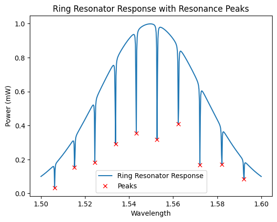
# Find resonance peaks
peaks = find_resonance_peaks(y, height=-0.01, distance=30, threshold=None)

y = spectrum

# Calculate FSR
fsr = calculate_FSR(x, peaks)

print("Resonance Peaks at:", x[peaks])
print("Free Spectral Range (FSR):", fsr)

plt.plot(x, y, label="Ring Resonator Response")
plt.plot(x[peaks], y[peaks], "x", color="red", label="Peaks")
plt.title("Ring Resonator Response with Resonance Peaks")
plt.xlabel("Wavelength")
plt.ylabel("Power (mW)")
plt.legend()
plt.show()

Resonance Peaks at: [1.50621242 1.51523046 1.5244489  1.53386774 1.54328657 1.55270541
 1.56232465 1.57214429 1.58216433 1.59218437]
Free Spectral Range (FSR): [0.00901804 0.00921844 0.00941884 0.00941884 0.00941884 0.00961924
 0.00981964 0.01002004 0.01002004]

def compute_group_index(wavelength, length, fsr):
    """Compute the group index (ng) of a ring resonator.

    Args:
        wavelength: Central wavelength of the resonator (in meters).
        length: Physical length of the ring resonator (in meters).
        fsr: Free Spectral Range (in meters).
    """
    ng = (wavelength**2) / (length * fsr)
    return ng


compute_group_index(x[peaks][:-1], 2 * np.pi * 10, fsr)

array([4.00387596, 3.96387755, 3.92688841, 3.97556304, 4.02453747,
       3.98894063, 3.95609914, 3.92586605, 3.97606843])

peaks.tolist()

[31, 76, 122, 169, 216, 263, 311, 360, 410, 460]

Generate wafer definitions

You can define different wafer maps for each wafer.

wafer_definitions = Path("wafer_definitions.json")
wafers = ["6d4c615ff105"]
wafer_attributes = dict(
    lot_id="lot1",
    attributes=dict(process_type="low_loss", wafer_diameter=200, wafer_thickness=0.7),
)

dies = [{"x": x, "y": y, "id": x * 8 + y} for y in range(0, 8) for x in range(0, 8)]

# Wrap in a list with the wafer information
data = [
    {"wafer": wafer_pkey, "dies": dies, **wafer_attributes} for wafer_pkey in wafers
]

with open(wafer_definitions, "w") as f:
    json.dump(data, f, indent=2)

Generate and write spectrums

You can easily generate some spectrum data and add some noise to make it look like a real measurement.

cwd = Path(".")

metadata = {"measurement_type": "Spectral MEAS", "temperature": 25}

noise_peak_to_peak_dB = 0.1
grating_coupler_loss_dB = 3
ng_noise = 0.1
length_variability = 1

for wafer in wafers:
    for die in dies:
        die = f"{(die['x'])}_{(die['y'])}"
        for (_, row), (_, device_row) in zip(df.iterrows(), df.iterrows()):
            cell_id = row["cell"]
            if "ridge" in cell_id:
                continue
            top_cell_id = "rings"
            device_id = f"{top_cell_id}_{cell_id}_{device_row['x']}_{device_row['y']}"
            dirpath = cwd / wafer / die / device_id
            dirpath.mkdir(exist_ok=True, parents=True)
            data_file = dirpath / "data.json"
            metadata_file = dirpath / "attributes.json"
            metadata_file.write_text(json.dumps(metadata))
            loss_dB = 2 * grating_coupler_loss_dB
            peak_power = 10 ** (-loss_dB / 10)
            grating_spectrum = np.array(
                [
                    gaussian_grating_coupler_response(
                        peak_power, center_wavelength, bandwidth_1dB, wl
                    )
                    for wl in wavelength_range
                ]
            )
            ring_spectrum = ring(
                wavelength_range,
                wl0=1.55,
                neff=2.4,
                ng=4.0 + ng_noise * np.random.rand(),
                ring_length=2 * np.pi * row["radius_um"]
                + length_variability * np.random.rand(),
                coupling=0.1,
                loss=30e2,  # 30 dB/cm = 30000 dB/m
            )
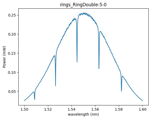
            output_power = grating_spectrum * ring_spectrum
            output_power *= 10 ** (
                noise_peak_to_peak_dB * np.random.rand(len(wavelength_range)) / 10
            )
            d = {
                "wavelength": wavelength_range * 1e3,
                "output_power": output_power,
                "polyfit": loss_dB,
            }
            data = pd.DataFrame(d)
            json_converted_file = data.reset_index(drop=True).to_dict(orient="split")
            json.dump(
                json_converted_file,
                open(data_file.with_suffix(".json"), "w+"),
                indent=2,
            )

plt.plot(wavelength_range, output_power)
plt.title(dirpath.stem)
plt.ylabel("Power (mW)")
plt.xlabel("wavelength (nm)")

Text(0.5, 0, 'wavelength (nm)')

f"{len(list(dirpath.parent.glob('*/*.json')))//2} measurements"

'9 measurements'

f"{len(list(dirpath.parent.parent.glob('*')))} dies"

'64 dies'