FDFD mode solver
We also have a FDFD mode solver.
Waveguides
Guided Electromagnetic modes are the ones that have an effective index larger than the cladding of the waveguide
Here is a waveguide of Silicon (n=3.4) surrounded by SiO2 (n=1.44) cladding
For a 220 nm height x 450 nm width the effective index is 2.466
# !uv add gdsfactory gplugins[tidy3d] # uncomment to install
# Config: filepaths, PDK activation, package imports and selected source
import gdsfactoryplus as gfp

pdk = gfp.get_pdk()
pdk.activate()
import gdsfactory as gf
import gplugins.tidy3d as gt
import matplotlib.pyplot as plt
import numpy as np
from gdsfactory.generic_tech import get_generic_pdk
import warnings

warnings.filterwarnings("ignore", category=FutureWarning, module="tidy3d")

gf.config.rich_output()
PDK = get_generic_pdk()
PDK.activate()

nm = 1e-3
wg_width = 0.5
wavelength = 1.55
core_thickness = 0.22
slab_thickness = 0.0
core_material = "si"  # can be a string or a number with the refractive index
clad_material = "sio2"

slab_thickness_rib = 0.15
nitride_thickness = 0.4

strip = gt.modes.Waveguide(
    wavelength=wavelength,
    core_width=wg_width,
    core_thickness=core_thickness,
    slab_thickness=slab_thickness,
    core_material=core_material,
    clad_material=clad_material,
    num_modes=2,
    sidewall_angle=np.deg2rad(10),
)

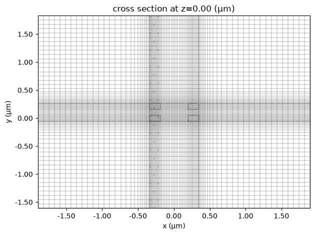
strip.plot_index()
plt.show()

21:21:32 UTC WARNING: The group index was not computed. To calculate group
             index, pass 'group_index_step = True' in the 'ModeSpec'.
# The field is exactly zero at some grid points, where its dB value is -inf.
with np.errstate(divide="ignore"):
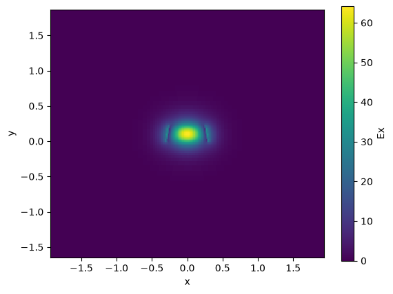
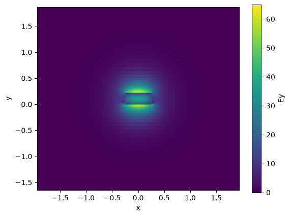
    strip.plot_field(field_name="Ex", mode_index=0, value="dB")  # TE
plt.show()
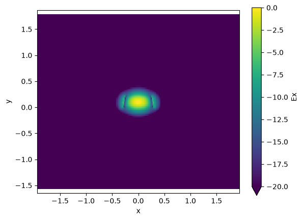
slab_thickness = 0.15

rib = gt.modes.Waveguide(
    wavelength=wavelength,
    core_width=wg_width,
    core_thickness=core_thickness,
    slab_thickness=slab_thickness,
    core_material=core_material,
    clad_material=clad_material,
    num_modes=2,
    sidewall_angle=np.deg2rad(10),
)

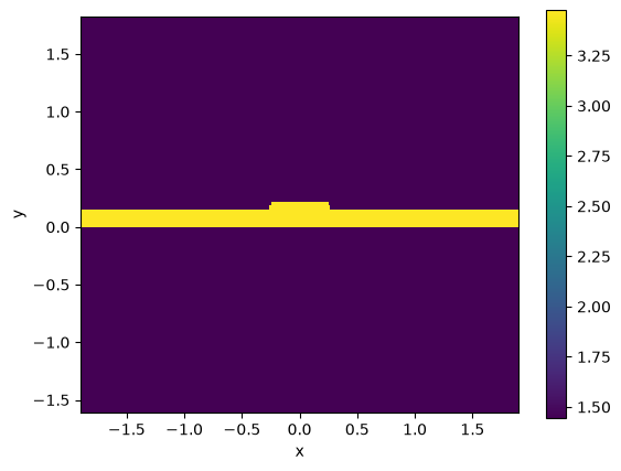
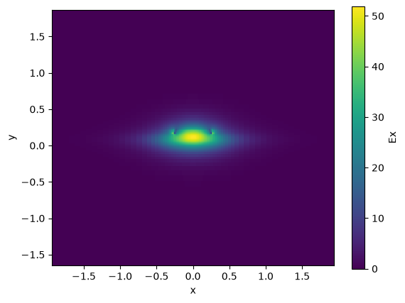
rib.plot_index()
rib.n_eff
21:21:33 UTC WARNING: Mode field at frequency index 0, mode index 1 does not
             decay at the plane boundaries.
nitride = gt.modes.Waveguide(
wavelength=wavelength,
core_width=1.0,
core_thickness=nitride_thickness,
slab_thickness=0.0,
core_material="sin", # can be a string or a number with the refractive index
clad_material="sio2",
sidewall_angle=np.deg2rad(10),
)
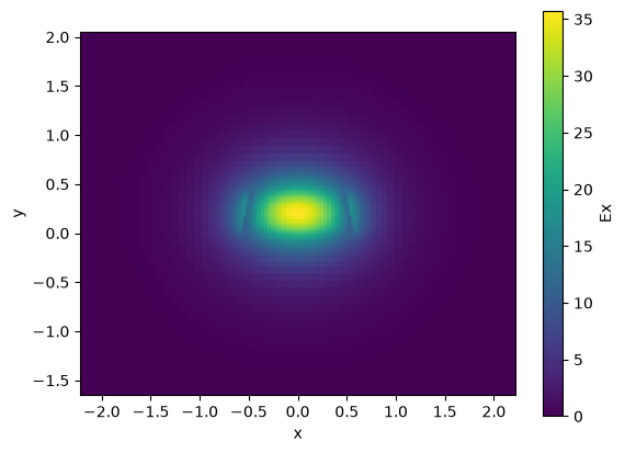
nitride.plot_index()
nitride.n_eff

Sweep width
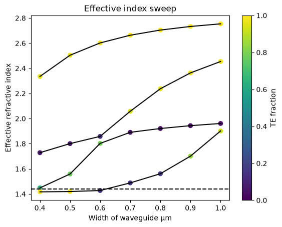
You can sweep the waveguide width and compute the modes.
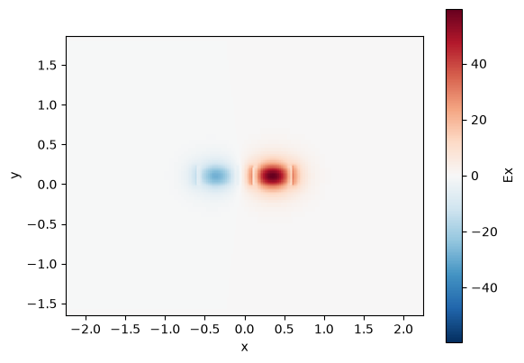
By increasing the waveguide width, the waveguide supports many more TE and TM modes. Where TE modes have a dominant Ex field and TM modes have larger Ey fields.
Notice that waveguides wider than 0.450 um support more than one TE mode. Therefore the maximum width for single mode operation is 0.450 um.
wg_width = 0.5
wavelength = 1.55
core_thickness = 0.22
slab_thickness = 0.0
core_material = "si" # can be a string or a number with the refractive index
clad_material = "sio2"
strip = gt.modes.Waveguide(
wavelength=wavelength,
core_width=wg_width,
core_thickness=core_thickness,
slab_thickness=slab_thickness,
core_material=core_material,
clad_material=clad_material,
num_modes=4,
sidewall_angle=np.deg2rad(10),
)
w = np.linspace(400 * nm, 1000 * nm, 7)
n_eff = gt.modes.sweep_n_eff(strip, core_width=w)
fraction_te = gt.modes.sweep_fraction_te(strip, core_width=w)
for i in range(4):
plt.plot(w, n_eff.sel(mode_index=i).real, c="k")
plt.scatter(
w, n_eff.sel(mode_index=i).real, c=fraction_te.sel(mode_index=i), vmin=0, vmax=1
)
plt.axhline(y=1.44, color="k", ls="--")
plt.colorbar().set_label("TE fraction")
plt.xlabel("Width of waveguide µm")
plt.ylabel("Effective refractive index")
plt.title("Effective index sweep")
plt.show()
21:21:36 UTC WARNING: Mode field at frequency index 0, mode index 3 does not decay at the plane boundaries.
21:21:37 UTC WARNING: Mode field at frequency index 0, mode index 3 does not decay at the plane boundaries.
Exercises
- What is the maximum width to support a single TE mode at 1310 nm?
- For a Silicon Nitride (n=2) 400nm thick waveguide surrounded by SiO2 (n=1.44), what is the maximum width to support a single TE mode at 1550 nm?
- For two 500x220nm Silicon waveguides surrounded by SiO2, what is the coupling length (100% coupling) for 200 nm gap?
Group index
You can also compute the group index for a waveguide.
nm = 1e-3
wavelength = 1.55
wg_width = 0.5
core_thickness = 0.22
strip = gt.modes.Waveguide(
wavelength=wavelength,
core_width=wg_width,
slab_thickness=0.0,
core_material="si",
clad_material="sio2",
core_thickness=core_thickness,
num_modes=4,
group_index_step=10 * nm,
)
print(strip.n_group)
21:21:44 UTC WARNING: Mode field at frequency index 0, mode index 3 does not decay at the plane boundaries.
WARNING: Mode field at frequency index 1, mode index 3 does not decay at the plane boundaries.
WARNING: Mode field at frequency index 2, mode index 3 does not decay at the plane boundaries.
Bend modes
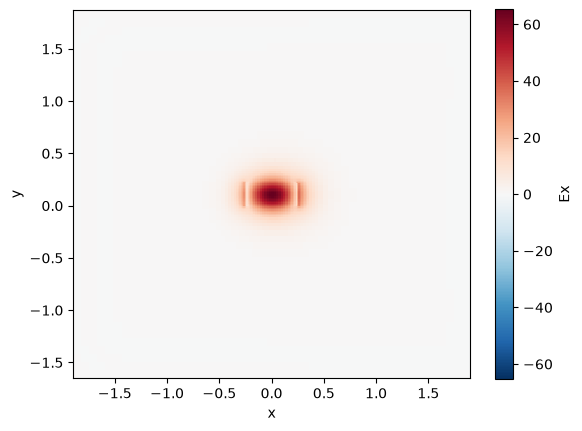
You can compute bend modes specifying the bend radius.
strip_bend = gt.modes.Waveguide(
wavelength=wavelength,
core_width=wg_width,
core_thickness=core_thickness,
slab_thickness=0.0,
bend_radius=4,
core_material="si",
clad_material="sio2",
)
strip_bend.plot_field(field_name="Ex", mode_index=0) # TE
plt.show()
21:21:45 UTC WARNING: Mode field at frequency index 0, mode index 1 does not decay at the plane boundaries.
Bend loss
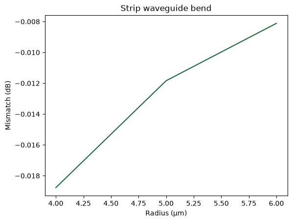
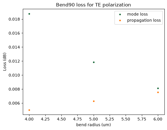
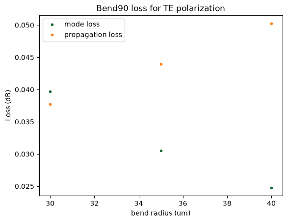
You can also compute the losses coming from the mode mismatch from the bend into a straight waveguide. To compute the bend loss due to mode mismatch you can calculate the mode overlap of the straight mode and the bent mode. Because there are two mode mismatch interfaces the total loss due to mode mismatch will be squared (from bend to straight and from straight to bend).

radii = np.arange(4, 7)
bend = gt.modes.Waveguide(
wavelength=wavelength,
core_width=wg_width,
core_thickness=core_thickness,
core_material="si",
clad_material="sio2",
num_modes=1,
bend_radius=radii.min(),
)
mismatch = gt.modes.sweep_bend_mismatch(bend, radii)
plt.plot(radii, 10 * np.log10(mismatch))
plt.title("Strip waveguide bend")
plt.xlabel("Radius (μm)")
plt.ylabel("Mismatch (dB)")
plt.show()
dB_cm = 2 # dB/cm
length = 2 * np.pi * radii * 1e-6
propagation_loss = dB_cm * length * 1e2
print(f"Propagation loss for 2πR bend: {propagation_loss} dB")
plt.title("Bend90 loss for TE polarization")
plt.plot(radii, -10 * np.log10(mismatch), ".", label="mode loss")
plt.plot(radii, propagation_loss, ".", label="propagation loss")
plt.xlabel("bend radius (um)")
plt.ylabel("Loss (dB)")
plt.legend()
plt.show()
rib = gt.modes.Waveguide(
wavelength=wavelength,
core_width=wg_width,
core_thickness=core_thickness,
slab_thickness=slab_thickness_rib,
bend_radius=15,
core_material="si",
clad_material="sio2",
)
rib.plot_field(field_name="Ex", mode_index=0)  # TE
plt.show()
21:21:49 UTC WARNING: Mode field at frequency index 0, mode index 0 does not
             decay at the plane boundaries.
             WARNING: Mode field at frequency index 0, mode index 1 does not
             decay at the plane boundaries.

nitride_bend = gt.modes.Waveguide(
    wavelength=1.55,
    core_width=1000 * nm,
    core_thickness=nitride_thickness,
    slab_thickness=0.0,
    bend_radius=30,
    core_material="sin",
    clad_material="sio2",
)
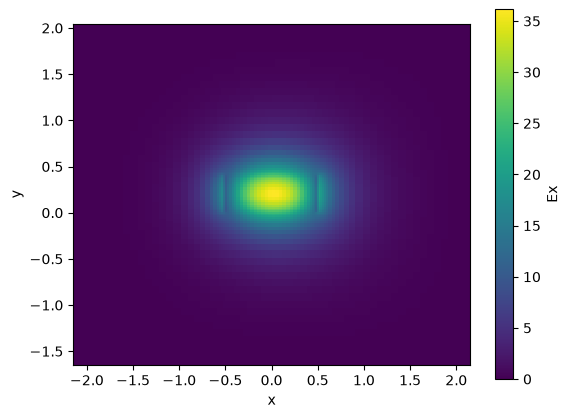
nitride_bend.plot_field(field_name="Ex", mode_index=0, value="abs")  # TE
plt.show()
radii = np.array([30, 35, 40])
bend = gt.modes.Waveguide(
    wavelength=wavelength,
    core_width=1000 * nm,
    core_thickness=nitride_thickness,
    core_material="sin",
    clad_material="sio2",
    num_modes=1,
    bend_radius=radii.min(),
)
mismatch = gt.modes.sweep_bend_mismatch(bend, radii)
dB_cm = 2  # dB/cm
length = 2 * np.pi * radii * 1e-6
propagation_loss = dB_cm * length * 1e2
print(f"propagation_loss for 2PI degree bend = {propagation_loss} dB")

plt.title("Bend90 loss for TE polarization")
plt.plot(radii, -10 * np.log10(mismatch), ".", label="mode loss")
plt.plot(radii, propagation_loss, ".", label="propagation loss")
plt.xlabel("bend radius (um)")
plt.ylabel("Loss (dB)")
plt.legend()
plt.show()
Exercises
- For a 500nm wide 220nm thick Silicon waveguide surrounded by SiO2, what is the minimum bend radius to have less than 0.04dB loss for TE polarization at 1550nm?
- For a 500nm wide 220nm thick Silicon waveguide surrounded by SiO2, what is the minimum bend radius to have 99% power transmission for TM polarization at 1550nm?
Waveguide coupler
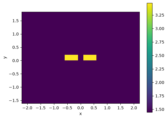
You can also compute the modes of a waveguide coupler.
       ore_width[0]  core_width[1]
        <------->     <------->
         _______       _______   _
        |       |     |       | |
        |       |     |       |
        |       |_____|       | | core_thickness
        |slab_thickness       |
        |_____________________| |_
                <----->
                  gap
gap = 200 * nm

c = gt.modes.WaveguideCoupler(
    wavelength=wavelength,
    core_width=(wg_width, wg_width),
    gap=gap,
    core_thickness=core_thickness,
    slab_thickness=slab_thickness,
    core_material="si",
    clad_material="sio2",
)
c.plot_index()
plt.show()
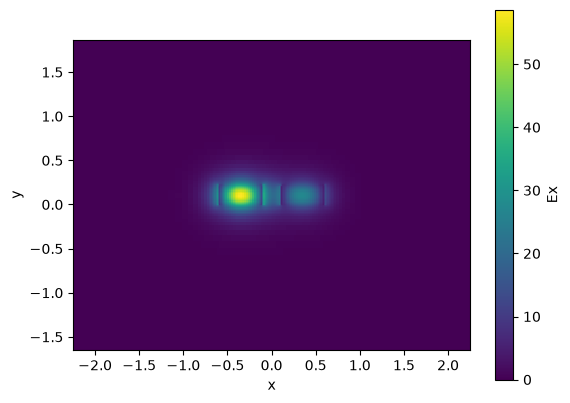
coupler = gt.modes.WaveguideCoupler(
    wavelength=wavelength,
    core_width=(wg_width, wg_width),
    gap=gap,
    core_thickness=core_thickness,
    slab_thickness=slab_thickness,
    core_material="si",
    clad_material="sio2",
    num_modes=4,
)

print("\nCoupler:", coupler)
print("Effective indices:", coupler.n_eff)
print("Mode areas:", coupler.mode_area)
print("Coupling length:", coupler.coupling_length())

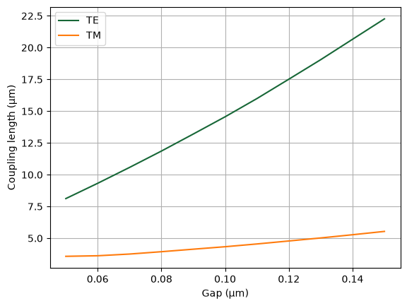
gaps = np.linspace(0.05, 0.15, 11)
lengths = gt.modes.sweep_coupling_length(coupler, gaps)

_, ax = plt.subplots(1, 1)
ax.plot(gaps, lengths)
ax.set(xlabel="Gap (μm)", ylabel="Coupling length (μm)")
ax.legend(["TE", "TM"])
ax.grid()
Coupler: WaveguideCoupler(wavelength=array(1.55), core_width=['0.5', '0.5'], core_thickness='0.22', core_material='si', clad_material='sio2', box_material=None, slab_thickness='0.0', clad_thickness=None, box_thickness=None, side_margin=None, sidewall_angle='0.0', sidewall_thickness='0.0', sidewall_k='0.0', surface_thickness='0.0', surface_k='0.0', bend_radius=None, target_neff=None, num_modes='4', group_index_step='False', precision='double', grid_resolution='20', max_grid_scaling='1.2', cache_path='/home/runner/.gdsfactory/modes', overwrite='False', gap='0.2')
Effective indices: [2.46849406+0.j 2.44315008+0.j 1.83051889+0.j 1.7207843 +0.j]
Mode areas: [0.27281044 0.26419291 0.6975965  0.64713647]
Coupling length: [30.57926254  7.06249486]