Running Palace Simulations¶

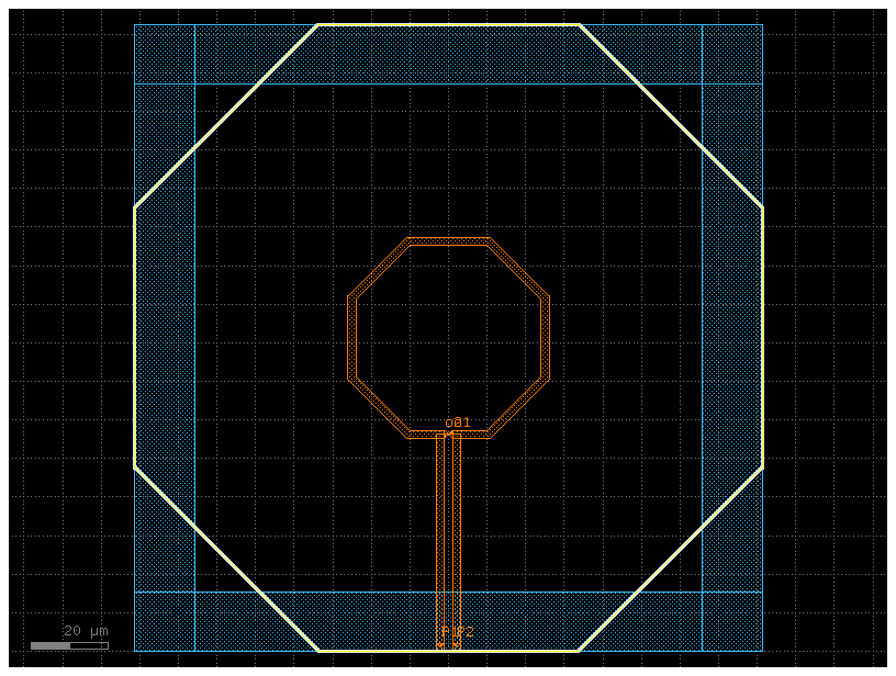
Palace is an open-source 3D electromagnetic simulator supporting eigenmode, driven (S-parameter), and electrostatic simulations. This notebook demonstrates using the gsim.palace API to run a driven simulation on a spiral inductor with Metal1 guard ring, and fitting the resulting S-parameters to an RLC equivalent circuit model for use in circulax.

Requirements: - IHP PDK: uv pip install ihp-gdsfactory - gsim with Palace backend - circulax: pip install circulax

Build inductor + guard ring¶

Known PDK limitation: gf.components.inductor accepts a turns parameter but does not use it in geometry construction. The spiral is always single-turn regardless of the value passed.

import gdsfactory as gf
from ihp import PDK

PDK.activate()

c = gf.components.inductor(
    width=2,
    space=2.1,
    diameter=50,
    turns=1,
    layer_metal="TopMetal2drawing",
    layer_inductor="INDdrawing",
    layer_metal_pin="TopMetal2drawing",
    layers_no_fill=("NoMetFillerdrawing",),
).copy()

# Define guard ring dimensions based on the inductor's bounding box
bbox = c.bbox()
xmin, ymin = bbox.left, bbox.bottom
xmax, ymax = bbox.right, bbox.top

margin_outer = 0.0
margin_inner = -15.0

xlo, xro = xmin - margin_outer, xmax + margin_outer
ybo, yto = ymin - margin_outer, ymax + margin_outer
xli, xri = xmin - margin_inner, xmax + margin_inner
ybi, yti = ymin - margin_inner, ymax + margin_inner

w_v = xli - xlo  # Width vertical walls
h_h = yto - yti  # Height horizontal walls
over = 0.5  # Overlap for Gmsh to fuse the pieces

# Left wall
c.add_ref(
    gf.components.rectangle(
        size=(w_v + over, yto - ybo), layer="Metal1drawing", centered=True
    )
).move((xlo + w_v / 2 + over / 2, (yto + ybo) / 2))
# Right wall
c.add_ref(
    gf.components.rectangle(
        size=(w_v + over, yto - ybo), layer="Metal1drawing", centered=True
    )
).move((xro - w_v / 2 - over / 2, (yto + ybo) / 2))
# Top wall
c.add_ref(
    gf.components.rectangle(
        size=(xro - xlo, h_h + over), layer="Metal1drawing", centered=True
    )
).move(((xro + xlo) / 2, yto - h_h / 2 - over / 2))
# Bottom wall
c.add_ref(
    gf.components.rectangle(
        size=(xro - xlo, h_h + over), layer="Metal1drawing", centered=True
    )
).move(((xro + xlo) / 2, ybo + h_h / 2 + over / 2))

cc = c.copy()

c.draw_ports()
c.plot()

png

Configure and run simulation with DrivenSim¶

from gsim.palace import DrivenSim

# Create simulation object
sim = DrivenSim()

# Set output directory
sim.set_output_dir("./palace-sim-inductor")

# Set the component geometry
sim.set_geometry(cc)

# Configure layer stack from active PDK
sim.set_stack(substrate_thickness=180.0, include_substrate=True)

# Configure ports
sim.add_port(
    "P1", from_layer="metal1", to_layer="topmetal2", geometry="via", excited=True
)
sim.add_port(
    "P2", from_layer="metal1", to_layer="topmetal2", geometry="via", excited=True
)

# Configure driven simulation (frequency sweep for S-parameters)
sim.set_driven(fmin=10e9, fmax=200e9, num_points=50)

# Validate configuration
print(sim.validate_config())

Validation: PASSED

# Generate mesh (presets: "coarse", "default", "fine")
sim.set_airbox(margin_x=50, margin_y=50, z_above=50, z_below=5)
sim.mesh(preset="default", refined_mesh_size=1.5)

Small conductor feature detected (2.100 um) may be under-resolved by refined_mesh_size=5.000 um. Pass auto_size=True to scale the mesh down.





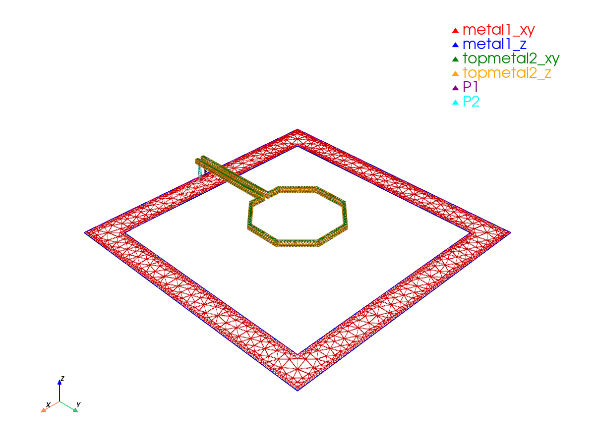
Mesh Summary
========================================
Dimensions: 362.6 x 362.6 x 250.9 µm
Nodes:      22,448
Elements:   167,880
Tetrahedra: 126,439
Edge length: 0.42 - 125.95 µm
Quality:    0.584 (min: 0.015)
SICN:       0.633 (all valid)
----------------------------------------
Volumes (4):
  - silicon [1]
  - sio2 [2]
  - sin [3]
  - air [4]
Surfaces (12):
  - metal1_xy [5]
  - metal1_z [6]
  - topmetal2_xy [7]
  - topmetal2_z [8]
  - P1 [9]
  - P2 [10]
  - air__silicon [11]
  - silicon__sio2 [12]
  - air__sio2 [13]
  - sin__sio2 [14]
  - air__sin [15]
  - air__None [16]
----------------------------------------
Mesh:   palace-sim-inductor/palace.msh

sim.plot_mesh(show_groups=["metal", "P"])

png

Run simulation on cloud¶

# Run simulation on GDSFactory+ cloud
results = sim.run()

  palace-33cd5b54  completed  3m 13s


Extracting results.tar.gz...
Downloaded 10 files to /home/runner/work/simulation-templates/simulation-templates/docs/notebooks/sim-data-palace-33cd5b54

results.plot_interactive()

Port mapping: Port 1: P1, Port 2: P2

results.plot_interactive(phase=True)

Port mapping: Port 1: P1, Port 2: P2

Analytical RLC Model Fit¶

Extract Differential Impedance¶

We assemble the S-parameter matrix from the simulation results into a scikit-rf Network object, which handles the conversion to Z-parameters. From the 2×2 Z-matrix we compute the differential impedance \(Z_\text{diff} = Z_{11} - Z_{12} - Z_{21} + Z_{22}\), which is the impedance seen between the two ports of the inductor under differential excitation.

import numpy as np
import skrf as rf

f = results.freq * 1e9  # GHz -> Hz
w = 2 * np.pi * f

ports = results.port_names
n = len(ports)

S = np.zeros((len(f), n, n), dtype=complex)
for i, pi in enumerate(ports):
    for j, pj in enumerate(ports):
        S[:, i, j] = results[(pi, pj)].complex

ntwk = rf.Network(f=f, s=S, f_unit="hz")
Z = ntwk.z

Z_sim = Z[:, 0, 0] - Z[:, 0, 1] - Z[:, 1, 0] + Z[:, 1, 1]
f_sim = f

RLC Model Definition¶

We fit an RLC equivalent circuit model to the simulated impedance data. The inductor is modeled as a series RL branch in parallel with a parasitic capacitance C:

RLC circuit

The total impedance is:

\[ Z(f) = \frac{1}{j2\pi f C + \frac{1}{R + j2\pi f L}} \]

We define the RLC impedance as a function of frequency. The total admittance (inverse of impedance) is the sum of the admittance of the series RL branch and the parasitic capacitance:

\[ \frac{1}{Z(f)} = \frac{1}{R + j2\pi f L} + j2\pi f C \]

We rewrite the RLC impedance in normalized form. Defining \(\tilde\omega = \omega/\omega_0\), the dimensionless impedance is:

\[ z(\tilde\omega, Q) = \frac{1 + j\tilde\omega Q}{1 - \tilde\omega^2 + j\tilde\omega/Q} \]

so that \(Z(f) = R \cdot z(f/f_0, Q)\).

The loss function measures the total squared error between the model and the simulated data across all frequencies:

\[ \mathcal{L}(f_0, Q, R) = \sum_k \left| Z_\text{sim}(f_k) - R \cdot z(f_k/f_0, Q) \right|^2 \]

This is a real-valued scalar that JAX will differentiate with respect to \(f_0\), \(Q\), and \(R\) to drive the optimization.

import jax
import jax.numpy as jnp

jax.config.update("jax_enable_x64", True)


# The RLC impedance function
def z_rlc(w, Q):
    return (1 + 1j * w * Q) / (1 - w**2 + 1j * w / Q)


f_jnp = jnp.array(f_sim, dtype=jnp.float64)
Z_target = jnp.array(Z_sim, dtype=jnp.complex128)


@jax.jit
def loss_fn(param):
    z_fit = param[2] * z_rlc(f_jnp / param[0], param[1])
    z_err = Z_target - z_fit
    return jnp.real(jnp.sum(z_err * jnp.conj(z_err)))

Initial Parameter Estimation¶

We estimate the initial values of \(R\), \(L\), and \(C\) directly from the data before running the optimization. Good initial values help the optimizer converge faster and avoid local minima.

\(f_0\) is read from the frequency at which \(|Z|\) is maximum
\(R \approx \text{Re}(Z)|_{f \to 0}\), the low-frequency resistance
\(Q\) is estimated from the -3 dB bandwidth: \(Q = f_0 / \Delta f\), where \(\Delta f\) is the width of the peak above \(|Z|_\text{max}/\sqrt{2}\)

absZ = np.abs(Z_sim)
f0_ini = float(f_sim[np.argmax(absZ)])
R_ini = float(Z_sim.real[0])
mask = absZ > np.max(absZ) / np.sqrt(2)
Q_ini = f0_ini / np.ptp(f_sim[mask]) if mask.sum() > 1 else 5.0
par_ini = jnp.array([f0_ini, Q_ini, R_ini])

print(f"f0 = {f0_ini / 1e9:.3f} GHz | Q = {Q_ini:.3f} | R = {R_ini:.4f} Ohm")

f0 = 168.980 GHz | Q = 5.000 | R = 0.9722 Ohm

Optimization¶

We minimize the squared error between the model and the data over all frequencies using the Adam optimizer.

At each step, Adam computes the gradient \(\nabla_\theta \mathcal{L}\) automatically via JAX autodiff and updates the parameters:

\[ \theta_{n+1} = \theta_n - \alpha \cdot \text{Adam}(\nabla_\theta \mathcal{L}(\theta_n)) \]

import optax

optimizer = optax.adam(learning_rate=0.05)
opt_state = optimizer.init(par_ini)
vg_fn = jax.jit(jax.value_and_grad(loss_fn))
vg_fn(par_ini)

par = par_ini
for step in range(1000):
    loss, grads = vg_fn(par)
    if step % 200 == 0:
        print(
            f"step {step:4d}: f0={float(par[0]) / 1e9:.4f} GHz  Q={float(par[1]):.3f}  R={float(par[2]):.4f}  loss={float(loss):.3e}"
        )
    updates, opt_state = optimizer.update(grads, opt_state)
    par = optax.apply_updates(par, updates)

f0_fit, Q_fit, R_fit = float(par[0]), float(par[1]), float(par[2])

step    0: f0=168.9796 GHz  Q=5.000  R=0.9722  loss=2.818e+07


step  200: f0=168.9796 GHz  Q=16.088  R=10.0037  loss=4.527e+06
step  400: f0=168.9796 GHz  Q=18.796  R=7.8604  loss=3.438e+06
step  600: f0=168.9796 GHz  Q=21.618  R=6.3505  loss=2.721e+06


step  800: f0=168.9796 GHz  Q=23.949  R=5.4361  loss=2.360e+06

Recover L and C¶

Once converged, \(L\) and \(C\) are recovered analytically from the fitted \((f_0, Q, R)\) using the RLC resonance relations:

\[ L = \frac{Q \cdot R}{\omega_0}, \quad C = \frac{1}{L\omega_0^2} \]

where \(\omega_0 = 2\pi f_0\).

w0 = 2 * np.pi * f0_fit
tau = Q_fit / w0
L_fit = tau * R_fit
C_fit = 1 / (L_fit * w0**2)

print(f"R = {R_fit:.6f} Ohm")
print(f"L = {L_fit * 1e12:.4f} pH")
print(f"C = {C_fit * 1e15:.4f} fF")
print(f"f0 = {f0_fit / 1e9:.4f} GHz  Q = {Q_fit:.3f}")

R = 4.878328 Ohm
L = 118.1184 pH
C = 7.5102 fF
f0 = 168.9796 GHz  Q = 25.708

Results¶

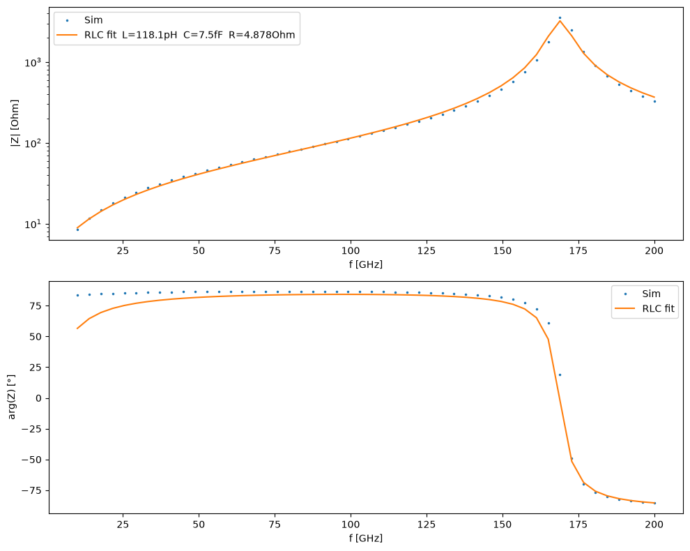
We evaluate the fitted model across the full frequency range and compare it against the simulation data. The two plots show the magnitude \(|Z(f)|\) on a log scale and the phase \(\arg(Z(f))\) in degrees — a good fit should reproduce both the inductive rise, the resonance peak, and the phase transition.

import matplotlib.pyplot as plt

print(f"\nR = {R_fit:.6f} Ohm")
print(f"L = {L_fit * 1e12:.4f} pH")
print(f"C = {C_fit * 1e15:.4f} fF")
print(f"f0 = {f0_fit / 1e9:.4f} GHz  Q = {Q_fit:.3f}")

Z_fit = np.array([R_fit * z_rlc(f / f0_fit, Q_fit) for f in f_sim])

fig, axes = plt.subplots(2, 1, figsize=(10, 8))
axes[0].plot(f_sim / 1e9, np.abs(Z_sim), ".", ms=3, label="Sim")
axes[0].plot(
    f_sim / 1e9,
    np.abs(Z_fit),
    label=f"RLC fit  L={L_fit * 1e12:.1f}pH  C={C_fit * 1e15:.1f}fF  R={R_fit:.3f}Ohm",
)
axes[0].set_yscale("log")
axes[0].set_xlabel("f [GHz]")
axes[0].set_ylabel("|Z| [Ohm]")
axes[0].legend()

axes[1].plot(f_sim / 1e9, np.angle(Z_sim, deg=True), ".", ms=3, label="Sim")
axes[1].plot(f_sim / 1e9, np.angle(Z_fit, deg=True), label="RLC fit")
axes[1].set_xlabel("f [GHz]")
axes[1].set_ylabel("arg(Z) [°]")
axes[1].legend()
plt.tight_layout()
plt.show()

R = 4.878328 Ohm
L = 118.1184 pH
C = 7.5102 fF
f0 = 168.9796 GHz  Q = 25.708

png

Circulax-Based Inverse Design¶

Define Circulax Component¶

With the fitted values from the analytical fit, we define my_inductor as a frequency-domain circulax component using @fdomain_component. The decorator converts the RLC admittance matrix into a two-port component compatible with any circulax netlist.

The admittance matrix for a symmetric two-port is:

\[ Y = \begin{pmatrix} Y_\text{tot} & -Y_\text{tot} \\ -Y_\text{tot} & Y_\text{tot} \end{pmatrix}, \quad Y_\text{tot} = \frac{1}{R + j2\pi f L} + j2\pi f C \]

The netlist connects the inductor directly between IN and GND — a single-port measurement configuration, consistent with how \(Z_\text{diff}\) was extracted from the simulation.

from circulax import compile_circuit
from circulax.s_transforms import fdomain_component

# Equivalent circuit:
#
#         --- C ---
#        |         |
# p1 ----+---R--L--+---- p2


@fdomain_component(ports=("p1", "p2"))
def my_inductor(f, R=1.0, L=100e-12, C=10e-15):
    w = 2.0 * jnp.pi * f
    Y_RL = 1.0 / (R + 1j * w * L)  # series RL branch
    Y_C = 1j * w * C  # parallel capacitance
    Y = Y_RL + Y_C
    return jnp.array([[Y, -Y], [-Y, Y]], dtype=jnp.complex128)


net_dict = {
    "instances": {
        "GND": {"component": "ground"},
        "L1": {
            "component": "my_inductor",
            "settings": {"R": R_fit, "L": L_fit, "C": C_fit},
        },
    },
    "connections": {
        "L1,p2": "GND,p1",
    },
    "ports": {
        "IN": "L1,p1",
    },
}

models = {"my_inductor": my_inductor, "ground": lambda: 0}

circuit = compile_circuit(net_dict, models)
groups = circuit.groups
freqs = jnp.asarray(f_sim)
Z_target = jnp.asarray(Z_sim)

print("Circuit compiled. System size:", circuit.sys_size)
print("Port map:", circuit.port_map)

Circuit compiled. System size: 2
Port map: {'IN': 1, 'L1,p1': 1, 'GND,p1': 0, 'L1,p2': 0}

Inverse Design with Circulax¶

We use circulax inside the optimization loop as part of a differentiable inverse design workflow. At each step, we perform a full AC sweep and minimize the discrepancy between the compact-model impedance and the Palace simulation data:

\[ \mathcal{L}(R,L,C) = \sum_k \left| Z_{\mathrm{target}}(f_k) - z_0 \frac{ 1 + S_{11}(f_k) }{ 1 - S_{11}(f_k) } \right|^2 \]

where the impedance is recovered from the simulated reflection coefficient through the standard one-port relation

\[ Z(f) = z_0 \frac{ 1 + S_{11}(f) }{ 1 - S_{11}(f) }. \]

The optimization is initialized using the analytical RLC fit parameters. To ensure physically meaningful values throughout the optimization, we optimize unconstrained variables and map them to positive parameters using a softplus parameterization:

\[ R,L,C > 0. \]

This enables stable gradient-based optimization using JAX automatic differentiation and Optax optimizers.

from circulax.solvers import setup_ac_sweep
from circulax.utils import update_params_dict

# Port node for IN — check port_map output above
port_node = next(v for k, v in circuit.port_map.items() if k == "IN")


# Positive parametrization
# raw_params -> softplus -> positive physical parameters
def positive(x):
    return jax.nn.softplus(x)


# inverse-softplus
def inv_softplus(y):
    return jnp.log(jnp.exp(y) - 1.0)


def loss_circulax(raw_params):
    params = positive(raw_params)
    R, L, C = params
    g = update_params_dict(groups, "my_inductor", "L1", "R", R)
    g = update_params_dict(g, "my_inductor", "L1", "L", L)
    g = update_params_dict(g, "my_inductor", "L1", "C", C)

    y_op = circuit.with_groups(g)()
    ac = setup_ac_sweep(groups=g, num_vars=circuit.sys_size, port_nodes=[port_node])
    sol = ac(freqs=freqs, y_dc=y_op)

    S11 = sol[:, 0, 0]
    Z_cx = 50.0 * (1 + S11) / (1 - S11)
    err_re = jnp.real(Z_cx) - jnp.real(Z_target)
    err_im = jnp.imag(Z_cx) - jnp.imag(Z_target)
    loss = jnp.mean(err_re**2 + err_im**2)

    return loss


raw_params_ini = inv_softplus(
    jnp.array(
        [
            R_fit,
            L_fit,
            C_fit,
        ]
    )
)

optimizer = optax.adam(1e-2)
opt_state = optimizer.init(raw_params_ini)
vg_fn = jax.jit(jax.value_and_grad(loss_circulax))
vg_fn(raw_params_ini)  # warm-up

raw_params = raw_params_ini
for step in range(500):
    loss, grads = vg_fn(raw_params)
    if step % 20 == 0:
        params = positive(raw_params)
        R_, L_, C_ = params
        print(
            f"step {step:3d}: R={float(R_):.5f} Ohm  L={float(L_) * 1e12:.3f} pH  C={float(C_) * 1e15:.3f} fF  loss={float(loss):.3e}"
        )
    updates, opt_state = optimizer.update(grads, opt_state)
    raw_params = optax.apply_updates(raw_params, updates)

R_fit_cx, L_fit_cx, C_fit_cx = [float(x) for x in positive(raw_params)]
f0_cx = 1.0 / (2 * np.pi * np.sqrt(L_fit_cx * C_fit_cx))
Q_cx = 2 * np.pi * f0_cx * L_fit_cx / R_fit_cx

print(f"\nR = {R_fit_cx:.6f} Ohm")
print(f"L = {L_fit_cx * 1e12:.4f} pH")
print(f"C = {C_fit_cx * 1e15:.4f} fF")
print(f"f0 = {f0_cx / 1e9:.4f} GHz  Q = {Q_cx:.3f}")

step   0: R=4.87833 Ohm  L=118.118 pH  C=7.550 fF  loss=7.845e+04
step  20: R=4.72177 Ohm  L=117.318 pH  C=7.473 fF  loss=6.830e+03
step  40: R=4.52897 Ohm  L=117.595 pH  C=7.451 fF  loss=4.296e+03
step  60: R=4.37351 Ohm  L=117.807 pH  C=7.439 fF  loss=2.999e+03
step  80: R=4.27276 Ohm  L=117.801 pH  C=7.441 fF  loss=2.573e+03
step 100: R=4.21909 Ohm  L=117.599 pH  C=7.455 fF  loss=2.412e+03
step 120: R=4.18966 Ohm  L=117.282 pH  C=7.475 fF  loss=2.270e+03
step 140: R=4.16548 Ohm  L=116.928 pH  C=7.498 fF  loss=2.124e+03
step 160: R=4.13937 Ohm  L=116.564 pH  C=7.521 fF  loss=1.979e+03
step 180: R=4.11133 Ohm  L=116.194 pH  C=7.545 fF  loss=1.835e+03
step 200: R=4.08271 Ohm  L=115.819 pH  C=7.570 fF  loss=1.696e+03
step 220: R=4.05413 Ohm  L=115.440 pH  C=7.595 fF  loss=1.561e+03
step 240: R=4.02575 Ohm  L=115.061 pH  C=7.620 fF  loss=1.432e+03
step 260: R=3.99765 Ohm  L=114.684 pH  C=7.645 fF  loss=1.309e+03
step 280: R=3.97000 Ohm  L=114.310 pH  C=7.670 fF  loss=1.195e+03
step 300: R=3.94294 Ohm  L=113.943 pH  C=7.695 fF  loss=1.088e+03
step 320: R=3.91656 Ohm  L=113.583 pH  C=7.720 fF  loss=9.886e+02


step 340: R=3.89096 Ohm  L=113.232 pH  C=7.744 fF  loss=8.975e+02
step 360: R=3.86622 Ohm  L=112.891 pH  C=7.767 fF  loss=8.141e+02
step 380: R=3.84238 Ohm  L=112.560 pH  C=7.790 fF  loss=7.384e+02
step 400: R=3.81950 Ohm  L=112.242 pH  C=7.812 fF  loss=6.699e+02
step 420: R=3.79760 Ohm  L=111.935 pH  C=7.834 fF  loss=6.084e+02
step 440: R=3.77671 Ohm  L=111.642 pH  C=7.854 fF  loss=5.534e+02
step 460: R=3.75683 Ohm  L=111.362 pH  C=7.874 fF  loss=5.045e+02
step 480: R=3.73798 Ohm  L=111.095 pH  C=7.893 fF  loss=4.612e+02

R = 3.720134 Ohm
L = 110.8410 pH
C = 7.9113 fF
f0 = 169.9593 GHz  Q = 31.818

Results¶

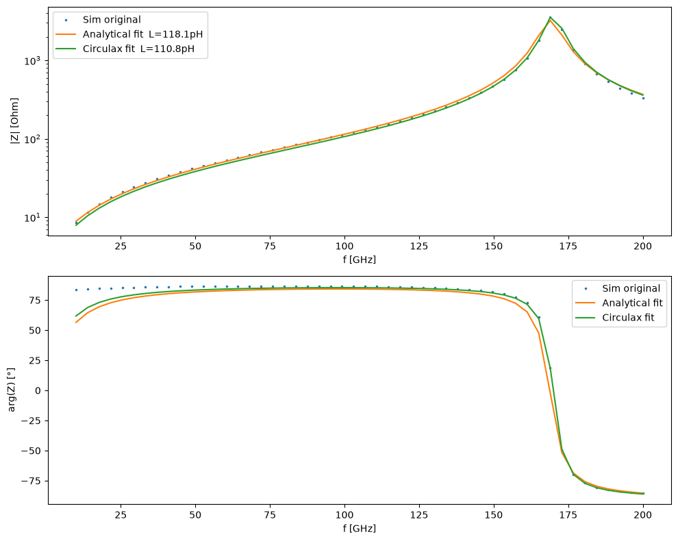
We compare the analytical fit and the circulax inverse design against the original simulation data.

g_final = update_params_dict(groups, "my_inductor", "L1", "R", R_fit_cx)
g_final = update_params_dict(g_final, "my_inductor", "L1", "L", L_fit_cx)
g_final = update_params_dict(g_final, "my_inductor", "L1", "C", C_fit_cx)

y_op_final = circuit.with_groups(g_final)()
ac_final = setup_ac_sweep(
    groups=g_final, num_vars=circuit.sys_size, port_nodes=[port_node]
)
sol_final = ac_final(freqs=freqs, y_dc=y_op_final)

S11_final = sol_final[:, 0, 0]
Z_cx_final = 50.0 * (1 + S11_final) / (1 - S11_final)

fig, axes = plt.subplots(2, 1, figsize=(10, 8))
axes[0].plot(f_sim / 1e9, np.abs(Z_sim), ".", ms=3, label="Sim original")
axes[0].plot(
    f_sim / 1e9, np.abs(Z_fit), label=f"Analytical fit  L={L_fit * 1e12:.1f}pH"
)
axes[0].plot(
    f_sim / 1e9, np.abs(Z_cx_final), label=f"Circulax fit  L={L_fit_cx * 1e12:.1f}pH"
)
axes[0].set_yscale("log")
axes[0].set_xlabel("f [GHz]")
axes[0].set_ylabel("|Z| [Ohm]")
axes[0].legend()

axes[1].plot(
    f_sim / 1e9, np.angle(np.array(Z_sim), deg=True), ".", ms=3, label="Sim original"
)
axes[1].plot(f_sim / 1e9, np.angle(np.array(Z_fit), deg=True), label="Analytical fit")
axes[1].plot(
    f_sim / 1e9, np.angle(np.array(Z_cx_final), deg=True), label="Circulax fit"
)
axes[1].set_xlabel("f [GHz]")
axes[1].set_ylabel("arg(Z) [°]")
axes[1].legend()
plt.tight_layout()
plt.show()

png