Directional coupler with GDSFactory FDTD
Run a 3D simulation using gsim.fdtd, a 50 nm Yee grid, and the active PDK. Exciting o1 returns one column of the S-matrix.
Requirements: gsim>=0.9.0 and GDSFactory+ cloud simulation access. To update an older project environment, run uv add "gsim>=0.9.0" "pdk-schema[sympy]~=0.3.0" from your project folder, then restart the notebook kernel.
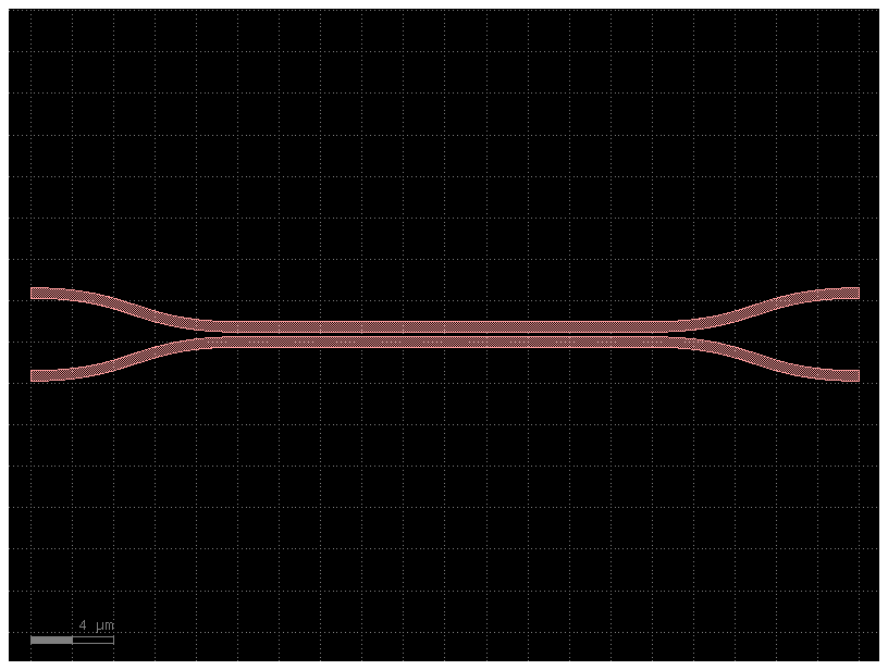
Load a component from the active PDK
import gdsfactory as gf

component = gf.get_component("coupler")
component = component.copy()
component.auto_rename_ports()
component
Configure the 3D simulation
Use the PDK layer stack with lossless silicon (n = 3.47) and silica (n = 1.44) at 1.55 µm. Sweep 1.50–1.60 µm; weak source-spectrum tails are hidden in the plots.
from gsim import fdtd

sim = fdtd.Simulation(pdk=pdk)
sim.materials(background="SiO2", overrides={"si": 3.47, "SiO2": 1.44})
sim.geometry(component=component, geometry_tolerance_nm=10)
sim.source(
    port="o1",
    wavelength_um=1.55,
    wavelength_span_um=0.1,
    num_wavelengths=101,
)
sim.domain(padding=1.0, pml_cells=20)
sim.solver(cell_size_nm=50, energy_decay_fraction=1e-6, max_wall_seconds=3600)
Inspect the geometry and record the field
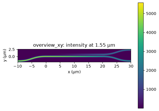
The interactive 3D view shows the device geometry and ports. An XY monitor through the input waveguide core records field intensity at the center wavelength, separately from the guided-port S-parameter monitors.
core_z_um = sim.resolved.ports[sim.source.port].center[2]
sim.monitors.add_plane(
    name="overview_xy",
    center_um=(component.dx, component.dy, core_z_um),
    size_um=(component.dxsize, component.dysize, 0),
    normal="+z",
    flux=False,
    heatmap=fdtd.Heatmap(quantity="intensity", wavelengths_um=[1.55]),
)

sim.plot_3d()
Inspect 2D cross-sections
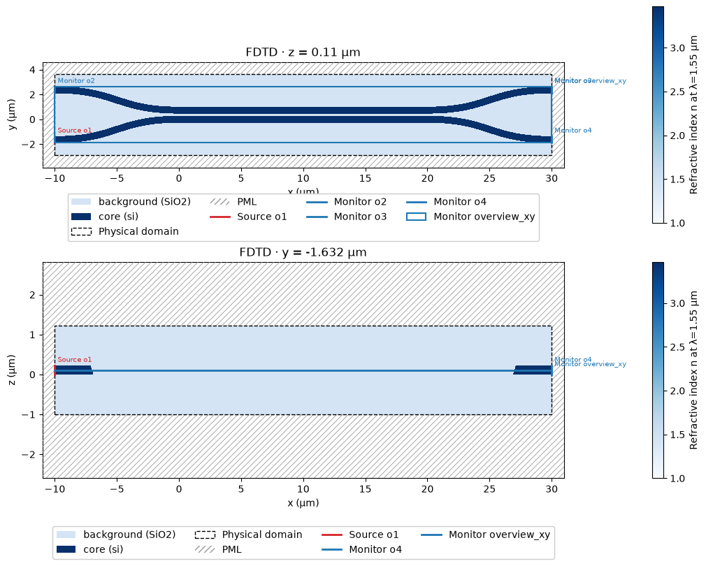
Static slices show the refractive index, the PML (hatched), the source, and the monitors the slice cuts. The XY slice passes through the waveguide core; the XZ slice runs along the input waveguide.
import matplotlib.pyplot as plt

port_y_um = sim.resolved.ports[sim.source.port].center[1]
fig, (ax_xy, ax_xz) = plt.subplots(2, 1, figsize=(10, 8), constrained_layout=True)
sim.plot_2d_static(axis="z", position_um=core_z_um, ax=ax_xy)
sim.plot_2d_static(axis="y", position_um=port_y_um, ax=ax_xz, aspect="auto")
plt.show()
Run on the cloud
Reuse a completed run when the simulation inputs match.
fdtd-70e5f8b6  [####################]  Job completed  elapsed 0m 00s
Extracting results.tar.gz...
Downloaded 3 files to /home/runner/work/simulation-templates/simulation-templates/docs/notebooks/sim-data-fdtd-70e5f8b6
Inspect the S-parameters
The two forward outputs share the input power. Their split depends on the coupling length and gap.
Field intensity
Use equal X and Y scales so a micrometer has the same displayed length in each direction.
field_figure, field_axis = result.monitors["overview_xy"].plot_heatmap(
    wavelength_um=sim.source.wavelength_um
)
field_axis.set_aspect("equal", adjustable="box")