Coupling to the continuum

Show code cell source

Hide code cell source

from collections import OrderedDict

import matplotlib.pyplot as plt
import numpy as np
import shapely
import shapely.affinity
from femwell.maxwell.waveguide import compute_modes
from femwell.mesh import mesh_from_OrderedDict
from femwell.visualization import plot_domains
from shapely.ops import clip_by_rect
from skfem import Basis, ElementDG, ElementTriP1
from skfem.io.meshio import from_meshio

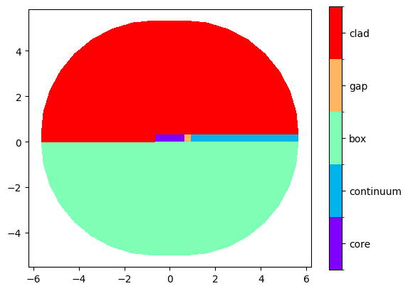
Let’s do a simple rectangular waveguide. Next to it we put a a slab of the same height and material, but wider, to which the field in the wavegudie couples. As we later add a PML to the simulation, this slab approximates an infinite wide wavegudie.

wg_width = 1.3
wg_thickness = 0.33
gap_width = 0.3
buffer = 5
pml_offset = 0.5
core = shapely.geometry.box(-wg_width / 2, 0, +wg_width / 2, wg_thickness)
gap = shapely.geometry.box(wg_width / 2, 0, +wg_width / 2 + gap_width, wg_thickness)
continuum = shapely.geometry.box(
    wg_width / 2 + gap_width, 0, +wg_width / 2 + buffer, wg_thickness
)
env = core.buffer(5, resolution=8)

polygons = OrderedDict(
    core=core,
    gap=gap,
    continuum=continuum,
    box=clip_by_rect(env, -np.inf, -np.inf, np.inf, 0),
    clad=clip_by_rect(env, -np.inf, 0, np.inf, np.inf),
)

resolutions = dict(
    core={"resolution": 0.05, "distance": 1},
    gap={"resolution": 0.05, "distance": 1},
    continuum={"resolution": 0.05, "distance": 1},
)

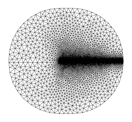
mesh = from_meshio(
    mesh_from_OrderedDict(polygons, resolutions, default_resolution_max=0.5)
)
mesh.draw().show()

plot_domains(mesh)
plt.show()

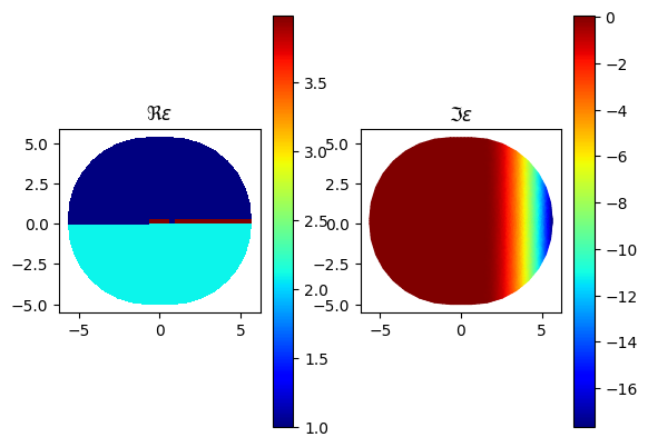
Now we define the epsilon! We add an PML on the right hand-side by adding an imaginary part to the epsilon.

basis0 = Basis(mesh, ElementDG(ElementTriP1()))
epsilon = basis0.zeros(dtype=complex)
for subdomain, n in {
    "core": 1.9963,
    "box": 1.444,
    "gap": 1.0,
    "continuum": 1.9963,
    "clad": 1,
}.items():
    epsilon[basis0.get_dofs(elements=subdomain)] = n**2
epsilon += basis0.project(
    lambda x: -1j * np.maximum(0, x[0] - (wg_width / 2 + gap_width + pml_offset)) ** 2,
    dtype=complex,
)
fig, axs = plt.subplots(1, 2)
for ax in axs:
    ax.set_aspect(1)
axs[0].set_title(r"$\Re\epsilon$")
basis0.plot(epsilon.real, colorbar=True, ax=axs[0])
axs[1].set_title(r"$\Im\epsilon$")
basis0.plot(epsilon.imag, shading="gouraud", colorbar=True, ax=axs[1])
plt.show()

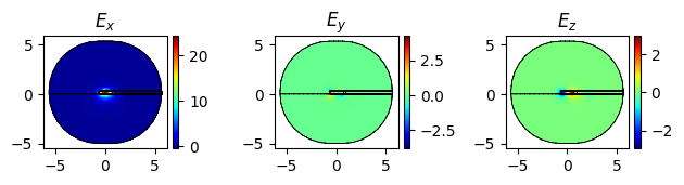
Now let’s calculate the mode of the wavegudie! We calculate the propagation loss from the imaginary part of the effective refractive index.

wavelength = 1.55

modes = compute_modes(basis0, epsilon, wavelength=wavelength, num_modes=1, order=1)
for mode in modes:
    print(
        f"Effective refractive index: {mode.n_eff:.12f}, "
        f"Loss: {mode.calculate_propagation_loss(distance=1):4f} / dB/um"
    )
    mode.plot(mode.E.real, colorbar=True, direction="x")
    plt.show()

Effective refractive index: 1.566634432079-0.000457954301j, Loss: 0.016124 / dB/um