Bent waveguide losses

This example uses an effective epsilon approximation for the bent, for more precise implementation see julia example.

Show code cell source

Hide code cell source

from collections import OrderedDict

import matplotlib.pyplot as plt
import numpy as np
from femwell.maxwell.waveguide import compute_modes
from femwell.mesh import mesh_from_OrderedDict
from shapely import box
from shapely.ops import clip_by_rect
from skfem import Basis, ElementDG, ElementTriP1
from skfem.io.meshio import from_meshio
from tqdm import tqdm

We describe the geometry using shapely. In this case it’s simple: we use a shapely.box for the waveguide. For the surrounding we buffer the core and clip it to the part below the waveguide for the box. The remaining buffer is used as the clad. For the core we set the resolution to 30nm and let it fall of over 500nm

wavelength = 1.55

wg_width = 0.5
wg_thickness = 0.22
slab_thickness = 0.11

core_index = 3.48
slab_index = 3.48

clad_index = 1.44
box_index = 1.44

pml_distance = wg_width / 2 + 2  # distance from center
pml_thickness = 2
core = box(-wg_width / 2, 0, wg_width / 2, wg_thickness)
slab = box(-1 - wg_width / 2, 0, pml_distance + pml_thickness, slab_thickness)
env = box(-1 - wg_width / 2, -1, pml_distance + pml_thickness, wg_thickness + 1)

polygons = OrderedDict(
    core=core,
    slab=slab,
    box=clip_by_rect(env, -np.inf, -np.inf, np.inf, 0),
    clad=clip_by_rect(env, -np.inf, 0, np.inf, np.inf),
)

resolutions = dict(
    core={"resolution": 0.03, "distance": 1}, slab={"resolution": 0.1, "distance": 0.5}
)

mesh = from_meshio(
    mesh_from_OrderedDict(
        polygons, resolutions, default_resolution_max=0.2, filename="mesh.msh"
    )
)
mesh.draw().show()

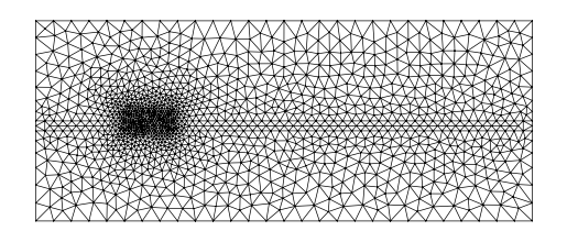
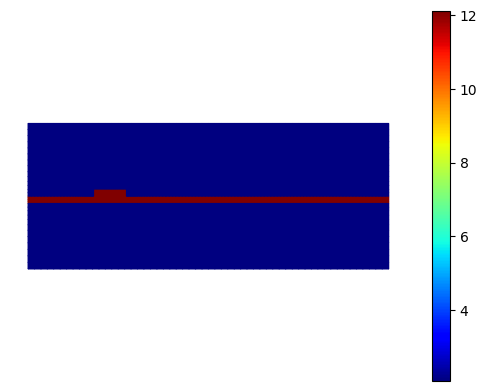
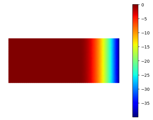
On this mesh, we define the epsilon. We do this by setting domainwise the epsilon to the squared refractive index. We additionally add a PML layer bt adding a imaginary part to the epsilon

basis0 = Basis(mesh, ElementDG(ElementTriP1()))
epsilon = basis0.zeros(dtype=complex)
for subdomain, n in {
    "core": core_index,
    "slab": slab_index,
    "box": box_index,
    "clad": clad_index,
}.items():
    epsilon[basis0.get_dofs(elements=subdomain)] = n**2
epsilon += basis0.project(
    lambda x: -10j * np.maximum(0, x[0] - pml_distance) ** 2,
    dtype=complex,
)
basis0.plot(epsilon.real, shading="gouraud", colorbar=True).show()
basis0.plot(epsilon.imag, shading="gouraud", colorbar=True).show()

We calculate now the modes for the geometry we just set up. We do it first for the case, where the bend-radius is infinite, i.e. a straight waveguide. This is done to have a reference effectie refractive index for starting and for mode overlap calculations between straight and bent waveguides.

modes_straight = compute_modes(
    basis0, epsilon, wavelength=wavelength, num_modes=1, order=2, radius=np.inf
)

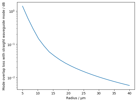
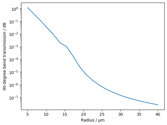
Now we calculate the modes of bent waveguides with different radii. Subsequently, we calculate the overlap integrals between the modes to determine the coupling efficiency And determine from the imaginary part the bend loss.

radiuss = np.linspace(40, 5, 21)
radiuss_lams = []
overlaps = []
lam_guess = modes_straight[0].n_eff
for radius in tqdm(radiuss):
    modes = compute_modes(
        basis0,
        epsilon,
        wavelength=wavelength,
        num_modes=1,
        order=2,
        radius=radius,
        n_guess=lam_guess,
        solver="scipy",
    )
    lam_guess = modes[0].n_eff
    radiuss_lams.append(modes[0].n_eff)

    overlaps.append(modes_straight[0].calculate_overlap(modes[0]))

And now we plot it!

Show code cell source

Hide code cell source

plt.xlabel("Radius / μm")
plt.ylabel("Mode overlap loss with straight waveguide mode / dB")
plt.yscale("log")
plt.plot(radiuss, -10 * np.log10(np.abs(overlaps) ** 2))
plt.show()
plt.xlabel("Radius / μm")
plt.ylabel("90-degree bend transmission / dB")
plt.yscale("log")
plt.plot(
    radiuss,
    -10
    * np.log10(
        np.exp(
            -2 * np.pi / wavelength * radius * np.abs(np.imag(radiuss_lams)) * np.pi / 2
        )
    ),
)
plt.show()

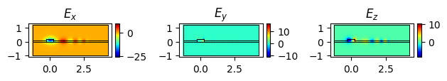
We now plot the mode calculated for the smallest bend radius to check that it’s still within the waveguide. As modes can have complex fields as soon as the epsilon gets complex, so we get a complex field for each mode. Here we show only the real part of the mode.

Show code cell source

Hide code cell source

for mode in modes:
    print(f"Effective refractive index: {mode.n_eff:.14f}")
    mode.plot(mode.E.real, colorbar=True, direction="x")
    plt.show()

Effective refractive index: 2.64348503506180-0.00848240209447j