Finite-element mode solver#
You can mesh any waveguide cross-section and solve for the optical modes using femwell.
This example defines a simple strip waveguide geometry using shapely, meshes it with femwell, and computes and visualizes the guided modes.
# !uv add femwell  # uncomment to install
#! uvx inc run gmsh
from collections import OrderedDict

import numpy as np
from femwell.maxwell.waveguide import compute_modes
from femwell.mesh import mesh_from_OrderedDict
from shapely.geometry import box
from shapely.ops import clip_by_rect
from skfem import Basis, ElementTriP0
from skfem.io.meshio import from_meshio
Define waveguide geometry#
We describe the cross-section geometry using shapely. A strip waveguide is a rectangular core sitting on a box (substrate), surrounded by cladding.
wavelength = 1.55
wg_width = 1.0
wg_thickness = 0.22

core_index = 3.45
clad_index = 1.444
box_index = 1.444

core = box(-wg_width / 2, 0, wg_width / 2, wg_thickness)
polygons = OrderedDict(
    core=core,
    box=clip_by_rect(core.buffer(3.0, resolution=4), -np.inf, -np.inf, np.inf, 0),
    clad=clip_by_rect(core.buffer(3.0, resolution=4), -np.inf, 0, np.inf, np.inf),
)

resolutions = {"core": {"resolution": 0.02, "distance": 2}}
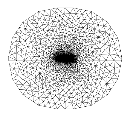
Generate mesh#
mesh = from_meshio(
    mesh_from_OrderedDict(
        polygons, resolutions, default_resolution_max=0.5, filename="mesh.msh"
    )
)
mesh.draw().show()
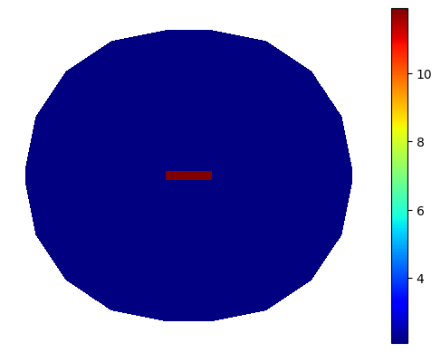
Assign material values#
basis0 = Basis(mesh, ElementTriP0())
epsilon = basis0.zeros()
for subdomain, n in {"core": core_index, "box": box_index, "clad": clad_index}.items():
    epsilon[basis0.get_dofs(elements=subdomain)] = n**2
basis0.plot(epsilon, colorbar=True).show()
Solve for modes#
modes = compute_modes(basis0, epsilon, wavelength=wavelength, num_modes=2, order=1)
Inspect modes#
You can use these as inputs to other femwell mode solver functions to inspect or analyze the modes.
print(f"Mode 0 TE fraction: {modes[0].te_fraction:.4f}")
print(f"Mode 1 TE fraction: {modes[1].te_fraction:.4f}")
Mode 0 TE fraction: 0.9978
Mode 1 TE fraction: 0.9874
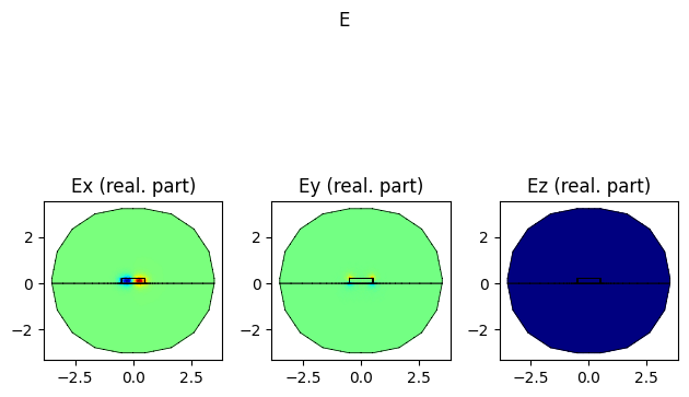
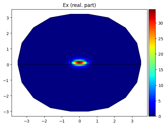
Plot electric field#
modes[0].show("E", part="real")
modes[0].plot_component("E", component="x", part="real", colorbar=True)
<Axes: title={'center': 'Ex (real. part)'}>
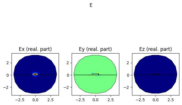
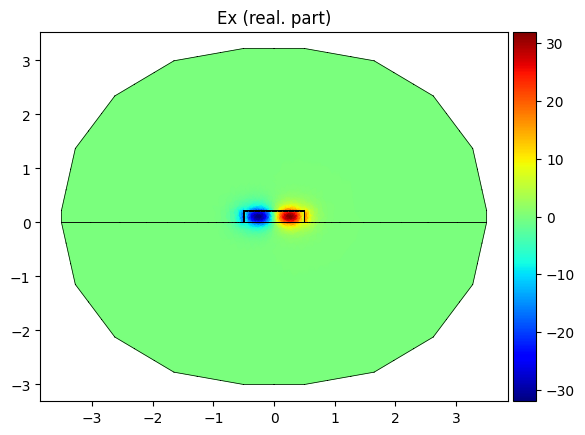
modes[1].plot_component("E", component="x", part="real", colorbar=True)
<Axes: title={'center': 'Ex (real. part)'}>
modes[1].show("E", part="real")