Circulax

A Differentiable, Functional Circuit Simulator based on JAX

Circulax is a differentiable circuit simulation framework built on JAX, Optimistix and Diffrax. It treats circuit netlists as systems of Ordinary Differential Equations (ODEs), leveraging Diffrax’s suite of numerical solvers for transient analysis.

The documentation can be found here

Why use JAX?

By using JAX as its backend, circulax provides:

Native Differentiation: Full support for forward and reverse-mode automatic differentiation through the solver, enabling gradient-based parameter optimization and inverse design.

Hardware Acceleration: Seamless execution on CPU, GPU, and TPU without code changes.

Mixed-Domain Support: Native complex-number handling for simultaneous simulation of electronic and photonic components.

Modular Architecture: A functional approach to simulation that integrates directly into machine learning and scientific computing workflows.

Standard tools (SPICE, Spectre, Ngspice) rely on established matrix stamping methods and CPU-bound sparse solvers. circulax leverages the JAX ecosystem to offer specific advantages in optimization and hardware utilization:

Feature	Legacy(SPICE)	circulax
Model Definition	Hardcoded C++ / Verilog-A	Simple python functions
Derivatives	Hardcoded (C) or Compiler-Generated (Verilog-A)	Automatic Differentiation (AD)
Solver Logic	Fixed-step or heuristic-based	Adaptive ODE stepping via Diffrax
Matrix Solver	Monolithic CPU Sparse (KLU)	Pluggable (KLUJAX, Dense, or Custom)
Hardware Target	CPU-bound	Agnostic (CPU/GPU/TPU)

Example LCR

import jax
import jax.numpy as jnp
import diffrax

import matplotlib.pyplot as plt

from circulax.compiler import compile_netlist
from circulax.components.electronic import Capacitor, Inductor, Resistor, VoltageSource
from circulax.solvers import analyze_circuit, setup_transient


net_dict = {
    "instances": {
        "GND": {"component": "ground"},
        "V1": {"component": "source_voltage", "settings": {"V": 1.0, "delay": 0.25e-9}},
        "R1": {"component": "resistor", "settings": {"R": 10.0}},
        "C1": {"component": "capacitor", "settings": {"C": 1e-11}},
        "L1": {"component": "inductor", "settings": {"L": 5e-9}},
    },
    "connections": {
        "GND,p1": ("V1,p2", "C1,p2"),
        "V1,p1": "R1,p1",
        "R1,p2": "L1,p1",
        "L1,p2": "C1,p1",
    },
}

import schemdraw
import schemdraw.elements as elm


# --- Helper for nice engineering labels ---
def get_formatted_label(instance_id):
    inst = net_dict["instances"][instance_id]
    comp_type = inst["component"]
    s = inst.get("settings", {})

    label = f"{instance_id}"

    if comp_type == "resistor":
        label += f"\n{s['R']}Ω"
    elif comp_type == "inductor":
        # Format scientific notation to prefixes (nH)
        val = s["L"]
        if val < 1e-6:
            label += f"\n{val * 1e9:.0f}nH"
        elif val < 1e-3:
            label += f"\n{val * 1e6:.0f}µH"
        else:
            label += f"\n{val}H"
    elif comp_type == "capacitor":
        # Format prefixes (pF, nF)
        val = s["C"]
        if val < 1e-9:
            label += f"\n{val * 1e12:.0f}pF"
        elif val < 1e-6:
            label += f"\n{val * 1e9:.0f}nF"
        else:
            label += f"\n{val}F"
    elif comp_type == "source_voltage":
        label += f"\n{s['V']}V Step"

    return label


# --- Drawing Routine ---
with schemdraw.Drawing() as d:
    d.config(
        fontsize=12, unit=3, inches_per_unit=0.7
    )  # Adjust unit size for better proportions

    V1 = d.add(elm.SourceV().up().label(get_formatted_label("V1")))

    R1 = d.add(
        elm.Resistor()
        .right()
        .at(V1.end)  # Connect to top of V1
        .label(get_formatted_label("R1"))
    )

    L1 = d.add(elm.Inductor().right().at(R1.end).label(get_formatted_label("L1")))
    C1 = d.add(elm.Capacitor().down().at(L1.end).label(get_formatted_label("C1")))

    d.add(elm.Line().to(V1.start))
    d.add(elm.Ground().at(V1.start))
    d.add(elm.Dot(open=True).at(V1.end).label("$V_{src}$", loc="top", color="blue"))
    d.add(elm.Dot(open=True).at(L1.end).label("$V_{cap}$", loc="top", color="blue"))

plt.rcParams.update({"axes.grid": True})
plt.style.use("dark_background")

jax.config.update("jax_enable_x64", True)


models_map = {
    "resistor": Resistor,
    "capacitor": Capacitor,
    "inductor": Inductor,
    "source_voltage": VoltageSource,
    "ground": lambda: 0,
}

print("Compiling...")
groups, sys_size, port_map = compile_netlist(net_dict, models_map)

print(port_map)

print(f"Total System Size: {sys_size}")
for g_name, g in groups.items():
    print(f"Group: {g_name}")
    print(f"  Count: {g.var_indices.shape[0]}")
    print(f"  Var Indices Shape: {g.var_indices.shape}")
    print(f"  Sample Var Indices:{g.var_indices}")
    print(f"  Jacobian Rows Length: {len(g.jac_rows)}")

print("2. Solving DC Operating Point...")
linear_strat = analyze_circuit(groups, sys_size, is_complex=False)

y_guess = jnp.zeros(sys_size)
y_op = linear_strat.solve_dc(groups, y_guess)

transient_sim = setup_transient(groups=groups, linear_strategy=linear_strat)
term = diffrax.ODETerm(lambda t, y, args: jnp.zeros_like(y))


t_max = 3e-9
saveat = diffrax.SaveAt(ts=jnp.linspace(0, t_max, 500))
print("3. Running Simulation...")
sol = transient_sim(
    t0=0.0,
    t1=t_max,
    dt0=1e-3 * t_max,
    y0=y_op,
    saveat=saveat,
    max_steps=100000,
    progress_meter=diffrax.TqdmProgressMeter(refresh_steps=100),
)

ts = sol.ts
v_src = sol.ys[:, port_map["V1,p1"]]
v_cap = sol.ys[:, port_map["C1,p1"]]
i_ind = sol.ys[:, 5]

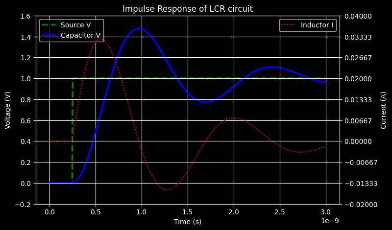
print("4. Plotting...")
fig, ax1 = plt.subplots(figsize=(8, 5))
ax1.plot(ts, v_src, "g--", linewidth=2.5, label="Source V")
ax1.plot(ts, v_cap, "b-", linewidth=2.5, label="Capacitor V")
ax1.set_xlabel("Time (s)")
ax1.set_ylabel("Voltage (V)")
ax1.legend(loc="upper left")

ax2 = ax1.twinx()
ax2.plot(ts, i_ind, "r:", label="Inductor I")
ax2.set_ylabel("Current (A)")
ax2.legend(loc="upper right")

ax2_ticks = ax2.get_yticks()
ax1_ticks = ax1.get_yticks()
ax2.set_yticks(jnp.linspace(ax2_ticks[0], ax2_ticks[-1], len(ax1_ticks)))
ax1.set_yticks(jnp.linspace(ax1_ticks[0], ax1_ticks[-1], len(ax1_ticks)))

plt.title("Impulse Response of LCR circuit")
plt.grid(True)
plt.show()

Compiling...
{'L1,p2': 1, 'C1,p1': 1, 'C1,p2': 0, 'GND,p1': 0, 'V1,p2': 0, 'R1,p2': 2, 'L1,p1': 2, 'V1,p1': 3, 'R1,p1': 3, 'V1,i_src': 4, 'L1,i_L': 5}
Total System Size: 6
Group: source_voltage
  Count: 1
  Var Indices Shape: (1, 3)
  Sample Var Indices:[[3 0 4]]
  Jacobian Rows Length: 1
Group: resistor
  Count: 1
  Var Indices Shape: (1, 2)
  Sample Var Indices:[[3 2]]
  Jacobian Rows Length: 1
Group: capacitor
  Count: 1
  Var Indices Shape: (1, 2)
  Sample Var Indices:[[1 0]]
  Jacobian Rows Length: 1
Group: inductor
  Count: 1
  Var Indices Shape: (1, 3)
  Sample Var Indices:[[2 1 5]]
  Jacobian Rows Length: 1
2. Solving DC Operating Point...

3. Running Simulation...

0.00%|          | [00:00<?, ?%/s]

0.10%|          | [00:00<00:05, 19.84%/s]

10.10%|█         | [00:00<00:00, 1322.30%/s]

20.10%|██        | [00:00<00:00, 1920.09%/s]

30.10%|███       | [00:00<00:00, 2279.14%/s]

40.10%|████      | [00:00<00:00, 2482.72%/s]

50.10%|█████     | [00:00<00:00, 2639.35%/s]

60.10%|██████    | [00:00<00:00, 2698.67%/s]

70.10%|███████   | [00:00<00:00, 2823.92%/s]

80.10%|████████  | [00:00<00:00, 2938.75%/s]

90.10%|█████████ | [00:00<00:00, 3037.67%/s]

100.00%|██████████| [00:00<00:00, 3105.53%/s]

4. Plotting...

Harmonic Balance

# Circuit parameters
R_val = 10.0  # Ω
L_val = 1e-6  # H  (1 µH)
C_val = 1e-9  # F  (1 nF)
V_amp = 1.0  # V (peak)

f_res = 1.0 / (2 * jnp.pi * jnp.sqrt(L_val * C_val))  # ≈ 5.033 MHz
Q = jnp.sqrt(L_val / C_val) / R_val  # ≈ 3.16
f_drive = f_res  # drive at resonance for maximum response

print(f"Resonant frequency : {f_res / 1e6:.3f} MHz")
print(f"Q-factor           : {Q:.3f}")
print(f"|H(jω₀)|           : {Q:.3f}  (capacitor voltage gain at resonance)")

Resonant frequency : 5.033 MHz
Q-factor           : 3.162
|H(jω₀)|           : 3.162  (capacitor voltage gain at resonance)

from circulax.components.electronic import VoltageSourceAC
from circulax import setup_harmonic_balance

# Netlist: Vs -> R -> L -> C -> GND
lcr_net = {
    "instances": {
        "Vs": {"component": "vsrc", "settings": {"V": V_amp, "freq": f_drive}},
        "R1": {"component": "resistor", "settings": {"R": R_val}},
        "L1": {"component": "inductor", "settings": {"L": L_val}},
        "C1": {"component": "capacitor", "settings": {"C": C_val}},
    },
    "connections": {
        "Vs,p1": "R1,p1",
        "R1,p2": "L1,p1",
        "L1,p2": "C1,p1",
        "C1,p2": "GND,p1",
        "Vs,p2": "GND,p1",
    },
    "ports": {"in": "Vs,p1", "out": "C1,p1"},
}

models = {
    "vsrc": VoltageSourceAC,
    "resistor": Resistor,
    "inductor": Inductor,
    "capacitor": Capacitor,
}

groups, num_vars, net_map = compile_netlist(lcr_net, models)
print(f"System size: {num_vars} variables")
print(f"Node map: {net_map}")

System size: 6 variables
Node map: {'L1,p2': 1, 'C1,p1': 1, 'C1,p2': 0, 'Vs,p2': 0, 'GND,p1': 0, 'R1,p2': 2, 'L1,p1': 2, 'R1,p1': 3, 'Vs,p1': 3, 'Vs,i_src': 4, 'L1,i_L': 5}

# DC operating point (zero for a purely AC circuit)
dc_solver = analyze_circuit(groups, num_vars, backend="dense")
y_dc = dc_solver.solve_dc(groups, jnp.zeros(num_vars))

# Harmonic Balance: 5 harmonics → K = 11 time points per period
N_harmonics = 5
run_hb = setup_harmonic_balance(
    groups, num_vars, freq=f_drive, num_harmonics=N_harmonics
)
y_time, y_freq = run_hb(y_dc)

print(
    f"y_time shape : {y_time.shape}  (K={2 * N_harmonics + 1} time points × {num_vars} variables)"
)
print(
    f"y_freq shape : {y_freq.shape}  ({N_harmonics + 1} harmonics × {num_vars} variables)"
)

y_time shape : (11, 6)  (K=11 time points × 6 variables)
y_freq shape : (6, 6)  (6 harmonics × 6 variables)

K = 2 * N_harmonics + 1
T = 1.0 / f_drive
t_ns = jnp.linspace(0, T * 1e9, K, endpoint=False)  # nanoseconds

vin_idx = net_map["Vs,p1"]
vout_idx = net_map["C1,p1"]

fig, ax = plt.subplots(figsize=(8, 3.5))
ax.plot(t_ns, jnp.array(y_time[:, vin_idx]), "C0o-", ms=6, label=r"$V_\mathrm{in}$")
ax.plot(t_ns, jnp.array(y_time[:, vout_idx]), "C1s-", ms=6, label=r"$V_\mathrm{out}$")
ax.set_xlabel("Time (ns)")
ax.set_ylabel("Voltage (V)")
ax.set_title("LCR — time-domain waveform (one period)")
ax.legend()
ax.grid(True, alpha=0.4)
plt.tight_layout()
plt.show()

# Two-sided amplitude: multiply by 2 for k≥1 (rfft folds negative frequencies)
harmonics = jnp.arange(N_harmonics + 1)
scale = jnp.where(harmonics == 0, 1.0, 2.0)
vin_amp = scale * jnp.abs(jnp.array(y_freq[:, vin_idx]))
vout_amp = scale * jnp.abs(jnp.array(y_freq[:, vout_idx]))
print(f"|V_in  @ f_drive| = {vin_amp[1]:.4f} V  (expected {V_amp:.4f} V)")
print(f"|V_out @ f_drive| = {vout_amp[1]:.4f} V  (expected Q={Q:.4f} V at resonance)")

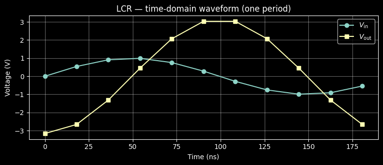
|V_in  @ f_drive| = 1.0000 V  (expected 1.0000 V)
|V_out @ f_drive| = 3.1623 V  (expected Q=3.1623 V at resonance)

freqs = jnp.logspace(5, 8, 500)  # 100 kHz → 100 MHz
w = 2 * jnp.pi * freqs
H = 1.0 / (1 - w**2 * L_val * C_val + 1j * w * R_val * C_val)

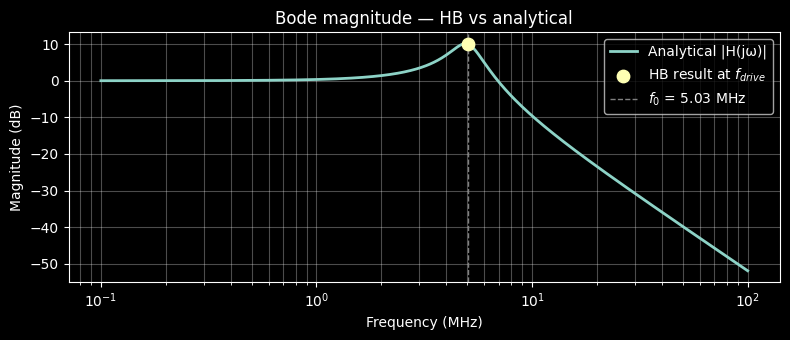
fig, ax = plt.subplots(figsize=(8, 3.5))
ax.semilogx(
    freqs / 1e6, 20 * jnp.log10(jnp.abs(H)), "C0", lw=2, label="Analytical |H(jω)|"
)
ax.scatter(
    [f_drive / 1e6],
    [20 * jnp.log10(vout_amp[1] / vin_amp[1])],
    color="C1",
    zorder=5,
    s=80,
    label="HB result at $f_{drive}$",
)
ax.axvline(
    f_res / 1e6, color="gray", ls="--", lw=1, label=f"$f_0$ = {f_res / 1e6:.2f} MHz"
)
ax.set_xlabel("Frequency (MHz)")
ax.set_ylabel("Magnitude (dB)")
ax.set_title("Bode magnitude — HB vs analytical")
ax.legend()
ax.grid(True, which="both", alpha=0.3)
plt.tight_layout()
plt.show()

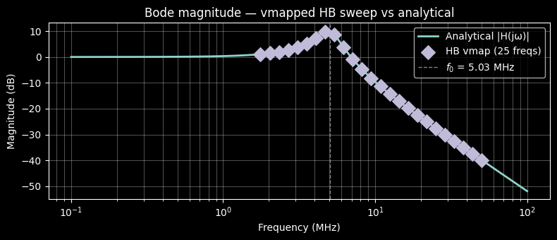
Frequency Sweep with jax.vmap

Because setup_harmonic_balance computes omega and t_points using standard JAX arithmetic, the entire HB solve — including the Newton loop — is vmappable over the drive frequency.

The pattern is:

def hb_solve_freq(freq):          # freq is now a JAX argument (i.e it is vectorized), not just a Python float
    run_hb = setup_harmonic_balance(groups, num_vars, freq=freq, ...)
    _, y_freq = run_hb(y_dc)
    return y_freq

y_freq_sweep = jax.jit(jax.vmap(hb_solve_freq))(sweep_freqs)

jax.vmap batches freq across the call — omega and t_points are derived per-element, and JAX lifts the Newton lax.while_loop to execute for all batch elements simultaneously. jax.jit then compiles the entire vectorised computation as a single XLA program.

# A thin wrapper that exposes freq as a JAX argument, making the function vmappable.
# groups and y_dc are captured by the outer closure and are shared across all frequencies.
def hb_solve_freq(freq):
    run_hb = setup_harmonic_balance(
        groups, num_vars, freq=freq, num_harmonics=N_harmonics
    )
    _, y_freq = run_hb(
        y_dc
    )  # y_dc is a non-batched free variable (same DC op-point for all freqs)
    return y_freq  # shape: (N_harmonics+1, num_vars)


# Five log-spaced frequencies spanning the LCR passband
sweep_freqs = jnp.geomspace(f_res * 0.35, f_res * 10.0, 25)
print("Sweep frequencies:", [f"{float(f) / 1e6:.3f} MHz" for f in sweep_freqs])

# jax.vmap maps the HB solve over all frequencies in a single XLA compilation.
# Internally, omega and t_points are computed from the batched freq axis, and the
# Newton loop (via optx.fixed_point / lax.while_loop) is lifted to handle the batch.
y_freq_sweep = jax.jit(jax.vmap(hb_solve_freq))(sweep_freqs)
# y_freq_sweep: shape (10, N_harmonics+1, num_vars)

# |H(jw)| = |V_out| / |V_in| at the fundamental (k=1)
H_hb_sweep = jnp.abs(y_freq_sweep[:, 1, vout_idx]) / jnp.abs(
    y_freq_sweep[:, 1, vin_idx]
)

# --- Plot against the analytical Bode curve ---
fig, ax = plt.subplots(figsize=(8, 3.5))
ax.semilogx(
    freqs / 1e6, 20 * jnp.log10(jnp.abs(H)), "C0", lw=2, label="Analytical |H(jω)|"
)
ax.scatter(
    jnp.array(sweep_freqs) / 1e6,
    20 * jnp.log10(jnp.array(H_hb_sweep)),
    color="C2",
    zorder=5,
    s=100,
    marker="D",
    label=f"HB vmap ({len(sweep_freqs)} freqs)",
)
ax.axvline(
    f_res / 1e6, color="gray", ls="--", lw=1, label=f"$f_0$ = {f_res / 1e6:.2f} MHz"
)
ax.set_xlabel("Frequency (MHz)")
ax.set_ylabel("Magnitude (dB)")
ax.set_title("Bode magnitude — vmapped HB sweep vs analytical")
ax.legend()
ax.grid(True, which="both", alpha=0.3)
plt.tight_layout()
plt.show()

print("\n|H(jω)| at sweep points:")
for f, Hv in zip(sweep_freqs, H_hb_sweep):
    w_rad = 2 * jnp.pi * float(f)
    H_exact = abs(1.0 / (1 - w_rad**2 * L_val * C_val + 1j * w_rad * R_val * C_val))
    print(
        f"  {float(f) / 1e6:.3f} MHz:  HB = {float(Hv):.4f},  analytical = {H_exact:.4f}"
    )

Sweep frequencies: ['1.762 MHz', '2.026 MHz', '2.329 MHz', '2.678 MHz', '3.080 MHz', '3.542 MHz', '4.073 MHz', '4.683 MHz', '5.385 MHz', '6.192 MHz', '7.121 MHz', '8.188 MHz', '9.416 MHz', '10.827 MHz', '12.450 MHz', '14.317 MHz', '16.463 MHz', '18.931 MHz', '21.769 MHz', '25.032 MHz', '28.785 MHz', '33.100 MHz', '38.062 MHz', '43.768 MHz', '50.329 MHz']

|H(jω)| at sweep points:
  1.762 MHz:  HB = 1.1306,  analytical = 1.1306
  2.026 MHz:  HB = 1.1798,  analytical = 1.1798
  2.329 MHz:  HB = 1.2511,  analytical = 1.2511
  2.678 MHz:  HB = 1.3582,  analytical = 1.3582
  3.080 MHz:  HB = 1.5273,  analytical = 1.5273
  3.542 MHz:  HB = 1.8126,  analytical = 1.8126
  4.073 MHz:  HB = 2.3272,  analytical = 2.3272
  4.683 MHz:  HB = 3.0922,  analytical = 3.0922
  5.385 MHz:  HB = 2.7169,  analytical = 2.7169
  6.192 MHz:  HB = 1.5515,  analytical = 1.5515
  7.121 MHz:  HB = 0.9115,  analytical = 0.9115
  8.188 MHz:  HB = 0.5796,  analytical = 0.5796
  9.416 MHz:  HB = 0.3892,  analytical = 0.3892
  10.827 MHz:  HB = 0.2709,  analytical = 0.2709
  12.450 MHz:  HB = 0.1931,  analytical = 0.1931
  14.317 MHz:  HB = 0.1399,  analytical = 0.1399
  16.463 MHz:  HB = 0.1025,  analytical = 0.1025
  18.931 MHz:  HB = 0.0757,  analytical = 0.0757
  21.769 MHz:  HB = 0.0563,  analytical = 0.0563
  25.032 MHz:  HB = 0.0420,  analytical = 0.0420
  28.785 MHz:  HB = 0.0315,  analytical = 0.0315
  33.100 MHz:  HB = 0.0236,  analytical = 0.0236
  38.062 MHz:  HB = 0.0178,  analytical = 0.0178
  43.768 MHz:  HB = 0.0134,  analytical = 0.0134
  50.329 MHz:  HB = 0.0101,  analytical = 0.0101

When to use s-parameters vs harmonic balance

S-parameters are used to represent linear components which means that it does not matter what the input signals are like, the output reponse is known. As this harmonic balance implmementation requires at minimum 2K+1 sample points per frequency it means that the matrix to solve becomes a dense f x 2K+1 x n_components matrix which is managable for small-medium circuits but might struggle for larger systems. Use SAX if all your components are linear. Use circulax for more general circuits

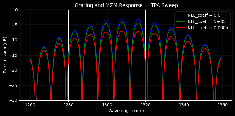
Example: Non-linear optical waveguide

dl = 50.0
d_inner = 100
d_in = 5000
d_out = d_in
d_out = d_in

net_dict = {
    "instances": {
        "GND": {"component": "ground"},
        "Laser": {"component": "source", "settings": {"power": 20.0, "phase": 0.0}},
        # Input Coupling
        "GC_In": {
            "component": "grating",
            "settings": {"peak_loss_dB": 1.0, "bandwidth_1dB": 40},
        },
        "WG_In": {"component": "waveguide", "settings": {"length_um": d_in}},
        # The Interferometer
        "Splitter": {"component": "splitter", "settings": {"split_ratio": 0.5}},
        "WG_Long": {
            "component": "waveguide",
            "settings": {"length_um": d_inner + dl},
        },  # Delta L = 100um
        "WG_Short": {"component": "waveguide", "settings": {"length_um": d_inner}},
        "Combiner": {
            "component": "splitter",
            "settings": {"split_ratio": 0.5},
        },  # Reciprocal Splitter
        # Output Coupling
        "WG_Out": {"component": "waveguide", "settings": {"length_um": d_out}},
        "GC_Out": {
            "component": "grating",
            "settings": {"peak_loss_dB": 1.0, "bandwidth_1dB": 40},
        },
        "Detector": {"component": "resistor", "settings": {"R": 1.0}},
    },
    "connections": {
        "GND,p1": ("Laser,p2", "Detector,p2"),
        # Input: Laser -> GC -> WG -> Splitter
        "Laser,p1": "GC_In,grating",
        "GC_In,waveguide": "WG_In,p1",
        "WG_In,p2": "Splitter,p1",
        # Arms
        "Splitter,p2": "WG_Long,p1",
        "Splitter,p3": "WG_Short,p1",
        "WG_Long,p2": "Combiner,p2",
        "WG_Short,p2": "Combiner,p3",
        # Output: Combiner -> WG -> GC -> Detector
        "Combiner,p1": "WG_Out,p1",
        "WG_Out,p2": "GC_Out,waveguide",
        "GC_Out,grating": "Detector,p1",
    },
}

from circulax.s_transforms import s_to_y
from circulax.components.base_component import PhysicsReturn, Signals, States, component


@component(ports=("p1", "p2"))
def OpticalWaveguideNL(
    signals: Signals,
    s: States,
    length_um: float = 100.0,
    loss_dBpercm: float = 1.0,
    nll_coefficient: float = 0.0,
    n_eff: float = 2.6,
    n_g: float = 4.06,
    center_wavelength_nm: float = 1310.0,
    wavelength_nm: float = 1310.0,
) -> PhysicsReturn:
    """
    Optical waveguide with linear loss, group-velocity dispersion, and
    power-dependent nonlinear loss (e.g. TPA / free-carrier effects).

    Linear propagation uses the group-index beta model:
        beta = 2π * (n_g / λ + (n_eff - n_g) / λ_0)
        s21_linear = 1j * exp(-(α/2 + i·beta) * L)

    Nonlinear loss is applied as an additional field-amplitude factor:
        nl_loss = 1 / sqrt(1 + 2 * nll_coefficient * L_mm * P_total²)
    where P_total = |V_p1|² + |V_p2|² and L_mm is the length in millimetres.

    nll_coefficient units: 1 / (W² · mm)
    """
    length_m = length_um * 1e-6

    # --- Linear propagation ---
    # Field attenuation coefficient: α_field = α_power / 2
    loss_dB_m = 100.0 * loss_dBpercm
    loss_power_m = (jnp.log(10.0) / 10.0) * loss_dB_m
    loss_field_m = 0.5 * loss_power_m

    # Propagation constant (group-index first-order dispersion model)
    lam_m = wavelength_nm * 1e-9
    lam0_m = center_wavelength_nm * 1e-9
    beta_m = 2.0 * jnp.pi * (n_g / lam_m + (n_eff - n_g) / lam0_m)

    # Complex propagation coefficient γ = α_field + i·beta
    gamma_m = loss_field_m + 1j * beta_m

    # Linear field transmission
    s21_linear = 1j * jnp.exp(-gamma_m * length_m)

    # --- Nonlinear loss ---
    # Total instantaneous power seen by the waveguide (both ports)
    p_total = jnp.abs(signals.p1) ** 2 + jnp.abs(signals.p2) ** 2
    length_mm = length_um * 1e-3  # convert µm → mm

    # nl_loss = 1 / sqrt(1 + 2 * nll_coefficient * L_mm * P_total²)
    # Written in numerically stable form matching the reference implementation:
    nl_loss = jnp.where(
        p_total > 0,
        1.0 / jnp.sqrt(p_total**-2 + 2.0 * nll_coefficient * length_mm) / p_total,
        1.0,
    )

    # Total field transmission = linear phase/loss × nonlinear field-amplitude factor
    T = jnp.sqrt(nl_loss) * s21_linear

    # --- S-matrix → Y-matrix → port currents ---
    # Waveguide is reciprocal: s12 = s21 = T, s11 = s22 = 0
    S = jnp.array([[0.0 + 0j, T], [T, 0.0 + 0j]], dtype=jnp.complex128)
    Y = s_to_y(S)
    v_vec = jnp.array([signals.p1, signals.p2], dtype=jnp.complex128)
    i_vec = Y @ v_vec

    return {"p1": i_vec[0], "p2": i_vec[1]}, {}

import time
import jax.numpy as jnp

from circulax.components.electronic import Resistor
from circulax.components.photonic import (
    Grating,
    OpticalSource,
    Splitter,
)
from circulax.compiler import compile_netlist
from circulax.solvers import analyze_circuit
from circulax.utils import update_group_params

import matplotlib.pyplot as plt

print("--- DEMO: Photonic Splitter & Grating Link (Wavelength + TPA Sweep) ---")

models_map = {
    "grating": Grating,
    "waveguide": OpticalWaveguideNL,
    "splitter": Splitter,
    "source": OpticalSource,
    "resistor": Resistor,
    "ground": lambda: 0,
}

groups, sys_size, port_map = compile_netlist(net_dict, models_map)

wavelengths = jnp.linspace(1260, 1360, 300)
nll_coeffs = jnp.array([0, 5e-5, 5e-4])

solver_strat = analyze_circuit(groups, sys_size, is_complex=True)


def solve_for_params(wavelength, tpa_coeff):
    g = update_group_params(groups, "grating", "wavelength_nm", wavelength)
    g = update_group_params(g, "waveguide", "wavelength_nm", wavelength)
    g = update_group_params(g, "waveguide", "nll_coefficient", tpa_coeff)
    y_flat = solver_strat.solve_dc(g, y_guess=jnp.ones(sys_size * 2))
    return y_flat


# Inner vmap: batches over tpa_coeff, holds wavelength fixed
solve_over_tpa = jax.vmap(solve_for_params, in_axes=(None, 0))
# Outer vmap: batches over wavelength, holds tpa_coeff array fixed
solve_2d = jax.vmap(solve_over_tpa, in_axes=(0, None))

print("Solving (JIT + vmap over wavelength × tpa_coeff)...")
start = time.time()
solutions_2d = jax.jit(solve_2d)(wavelengths, nll_coeffs)
total = time.time() - start
print(f"Total simulation time: {total:.3f}s")
# solutions_2d shape: (n_wavelengths, n_tpa_coeffs, sys_size * 2)

v_in = (
    solutions_2d[..., port_map["Laser,p1"]]
    + 1j * solutions_2d[..., port_map["Laser,p1"] + sys_size]
)
p_in_db = 10.0 * jnp.log10(jnp.abs(v_in) ** 2 + 1e-12)

v_out = (
    solutions_2d[..., port_map["Detector,p1"]]
    + 1j * solutions_2d[..., port_map["Detector,p1"] + sys_size]
)
p_out_db = 10.0 * jnp.log10(jnp.abs(v_out) ** 2 + 1e-12)
# p_out_db shape: (n_wavelengths, n_tpa_coeffs)

tpa_labels = [f"NLL_coeff = {x}" for x in nll_coeffs]
colors = ["b", "g", "r"]

plt.figure(figsize=(8, 4))
for i, (label, color) in enumerate(zip(tpa_labels, colors)):
    plt.plot(wavelengths, p_out_db[:, i] - p_in_db[:, i], color=color, label=label)

plt.title("Grating and MZM Response — TPA Sweep")
plt.xlabel("Wavelength (nm)")
plt.ylabel("Transmission (dB)")
plt.ylim(ymin=-30)
plt.legend()
plt.grid(True)
plt.tight_layout()
plt.show()

--- DEMO: Photonic Splitter & Grating Link (Wavelength + TPA Sweep) ---

Solving (JIT + vmap over wavelength × tpa_coeff)...

Total simulation time: 4.794s

Silicon Ring Modulator: Electro-Optic Simulation

This notebook simulates the transient optical response of a ring resonator modulator using Temporal Coupled-Mode Theory (t-CMT). An optical pulse is launched into a bus waveguide coupled to the ring. We observe how the ring energy \(a(t)\) builds up and decays, and how this shapes the transmitted field.

This notebook covers four progressively more complex analyses:

• Part 1 Optical impulse response: Step-on/off pulse excites the ring, revealing the photon lifetime \(\tau\).

• Part 2 Small-signal EO bandwidth (time-domain sweep): AC voltage drives a PN junction; transient simulation extracts the EO 3-dB bandwidth.

• Part 3 EO bandwidth via Harmonic Balance: Same bandwidth measurement using jax.vmap over frequency in a single JIT call.

• Part 4 Large-signal NRZ eye diagram: 128-bit PRBS pattern at 56 GBaud reveals ISI from photon-lifetime memory.

• Part 5 \(V_\mathrm{bias}\) sweep via jax.vmap: Four eye diagrams at different bias voltages, computed in a single vmapped transient call.

t-CMT equations

The complex ring energy \(a(t)\) (with \(|a|^2\) in units of energy) evolves as:

\[\frac{da}{dt} = -j\sqrt{\frac{2}{\tau_e}}\,E_i(t) + j\,\Delta\omega\,a(t) - \frac{a(t)}{\tau}\]

where \(\Delta\omega = 2\pi(f_{\rm op} - f_r) + V_{\rm wr}\,V\) is the laser\u2013resonance detuning, and \(1/\tau = 1/\tau_e + 1/\tau_l\) combines the coupling (\(\tau_e\)) and loss (\(\tau_l\)) photon lifetimes. The transmitted field is

\[E_o(t) = E_i(t) - j\sqrt{\frac{2}{\tau_e}}\,a(t).\]

Mapping to the circulax DAE (\(F + dQ/dt = 0\))

The RingModulator component below carries two internal states:

State	\(F\)-term (residual)	\(Q\)-term (storage)	Role
a	\(j\sqrt{2/\tau_e}\,V_{p1} - j\Delta\omega\,a + a/\tau\)	\(a\)	Ring energy ODE
i_out	\(V_{p2}-(V_{p1}-j\sqrt{2/\tau_e}\,a)\)	\u2014	Output field constraint

Port p1 (input) contributes zero current \u2014 the ring is transparent at the input (S11 = 0), so the source drives the input field directly. Port p2 (output) is driven by the auxiliary state i_out, which enforces the output field relation algebraically.

The ring energy can be recovered as a post-processing step directly from the port voltages: \(a = -j\,(E_i - E_o)/\sqrt{2/\tau_e}\).

---

References: Absil et al., OE 2000; Choi et al., OE 2015

import diffrax
import jax
import jax.numpy as jnp
import matplotlib.pyplot as plt
import numpy as np

from circulax.compiler import compile_netlist
from circulax.components.base_component import (
    PhysicsReturn,
    Signals,
    States,
    component,
    source,
)
from circulax.components.electronic import Resistor
from circulax.solvers import analyze_circuit, setup_transient

jax.config.update("jax_enable_x64", True)

Component definitions

@source(ports=("p1", "p2"), states=("i_src",))
def OpticalSourcePulseOnOff(
    signals: Signals,
    s: States,
    t: float,
    power: float = 1.0,
    phase: float = 0.0,
    t_on: float = 50e-12,
    t_off: float = 150e-12,
    rise: float = 5e-12,
) -> PhysicsReturn:
    """CW optical source with a smooth rectangular pulse envelope.

    Two sigmoid ramps (one up, one down) define the on/off transitions.
    The rise-time constant ``rise`` should be chosen small relative to the
    photon lifetime to approximate a sharp turn-on/off.

    Args:
        signals: Field amplitudes at positive (``p1``) and negative (``p2``) ports.
        s: Source current state variable ``i_src``.
        t: Simulation time.
        power: Peak optical power in watts. Defaults to ``1.0``.
        phase: Output field phase in radians. Defaults to ``0.0``.
        t_on: Turn-on time in seconds. Defaults to ``50e-12``.
        t_off: Turn-off time in seconds. Defaults to ``150e-12``.
        rise: Sigmoid rise/fall time constant. Defaults to ``5e-12``.

    """
    sigmoid_on = jax.nn.sigmoid((t - t_on) / rise)
    sigmoid_off = jax.nn.sigmoid((t - t_off) / rise)
    amp = jnp.sqrt(power) * jnp.exp(1j * phase) * (sigmoid_on - sigmoid_off)
    constraint = (signals.p1 - signals.p2) - amp
    return {"p1": s.i_src, "p2": -s.i_src, "i_src": constraint}, {}


@component(ports=("p1", "p2"), states=("a", "i_out"))
def RingModulator(
    signals: Signals,
    s: States,
    ng: float = 3.8,
    L: float = 3.14159265e-5,
    gamma: float = 0.976,
    alpha0: float = 0.969,
    alpha1: float = 0.0,
    voltage: float = 0.0,
    f_operating: float = 2.2904e14,
    f_resonance: float = 2.2901e14,
    v_to_wr: float = 0.0,
) -> PhysicsReturn:
    """Optical ring modulator via Temporal Coupled-Mode Theory (t-CMT).

    Tracks the complex ring energy amplitude ``a(t)`` as an internal state and
    enforces the output field relation ``E_o = E_i - j sqrt(2/tau_e) a`` via an
    algebraic constraint state ``i_out``.

    The ring energy ODE is expressed in the circulax DAE form F + dQ/dt = 0:

    - F["a"] = -(da/dt RHS) = j sqrt(2/tau_e) V_p1 - j Delta_omega a + a/tau
    - Q["a"] = a

    Gives: da/dt = -j sqrt(2/tau_e) E_i + j Delta_omega a - a/tau.

    Port ``p1`` contributes zero current (S11 = 0 approximation).
    Port ``p2`` is driven by ``i_out`` which enforces the output field.

    Args:
        signals: Complex field amplitudes at input (``p1``) and output (``p2``).
        s: Internal states: ``a`` (complex ring energy) and ``i_out`` (output
            constraint current).
        ng: Group refractive index. Defaults to ``3.8``.
        L: Ring circumference in metres. Defaults to ``2*pi*5e-6``.
        gamma: Through-coupling amplitude coefficient. Defaults to ``0.976``.
        alpha0: Voltage-independent round-trip amplitude. Defaults to ``0.969``.
        alpha1: Linear voltage coefficient of round-trip amplitude (1/V).
            Defaults to ``0.0``.
        voltage: Applied DC bias voltage. Defaults to ``0.0``.
        f_operating: Laser frequency in Hz. Defaults to ``2.2904e14``.
        f_resonance: Ring resonance frequency in Hz. Defaults to ``2.2901e14``.
        v_to_wr: Electro-optic coefficient mapping voltage to resonance shift
            in rad/s/V. Defaults to ``0.0``.

    """
    c = 2.998e8  # speed of light, m/s

    # Photon lifetimes
    tau_e = 2.0 * ng * L / ((1.0 - gamma**2) * c)
    alpha_v = alpha0 + alpha1 * voltage
    tau_l = 2.0 * ng * L / ((1.0 - alpha_v**2) * c)
    tau = 1.0 / (1.0 / tau_e + 1.0 / tau_l)

    coupling = jnp.sqrt(2.0 / tau_e)

    # Laser-resonance detuning (+ EO shift)
    delta_omega = 2.0 * jnp.pi * (f_operating - f_resonance) + v_to_wr * voltage

    # Ring energy ODE RHS: da/dt = -j*coupling*E_i + j*delta_omega*a - a/tau
    rhs_a = -1j * coupling * signals.p1 + 1j * delta_omega * s.a - s.a / tau

    # Output field from the ring: E_o = E_i - j*coupling*a
    E_o_expected = signals.p1 - 1j * coupling * s.a

    f = {
        "p1": 0.0 + 0.0j,  # ring is transparent at input (S11=0)
        "p2": s.i_out,
        "i_out": signals.p2 - E_o_expected,  # enforce E_o = E_i - j*coupling*a
        "a": -rhs_a,  # ring energy ODE (negated RHS)
    }
    q = {"a": s.a}
    return f, q

Simulation parameters

Parameters are taken from the reference silicon photonics ring modulator in Choi et al., OE 2015.

c = 2.998e8  # m/s

# Ring geometry and coupling
ng = 3.8
radius_um = 5.0  # ring radius, μm
L_ring = float(2.0 * np.pi * radius_um * 1e-6)  # circumference, m
gamma = 0.976  # through-coupling amplitude
alpha0 = 0.969  # round-trip amplitude (unbiased)

# Operating wavelength – 0.30 nm blue-detuned from resonance.
# This gives Δω·τ ≈ 2.4, producing ~1–2 visible ringing cycles during the
# ~3τ transient when the source turns on with a sharp (1 ps) rise time.
wavelength_res_nm = 1310.0
detuning_nm = 0.30
wavelength_op_nm = wavelength_res_nm - detuning_nm

f_resonance = c / (wavelength_res_nm * 1e-9)
f_operating = c / (wavelength_op_nm * 1e-9)

# Derived photon lifetimes
tau_e = 2.0 * ng * L_ring / ((1.0 - gamma**2) * c)
tau_l = 2.0 * ng * L_ring / ((1.0 - alpha0**2) * c)
tau = 1.0 / (1.0 / tau_e + 1.0 / tau_l)
coupling = np.sqrt(2.0 / tau_e)

# Ringing oscillation period: beats between laser and ring resonance
delta_f = f_operating - f_resonance
T_osc = 1.0 / delta_f  # period of output power oscillation during transient

# Steady-state transmission (analytic)
A = 2.0 * tau / tau_e
x = 2.0 * np.pi * delta_f * tau  # normalised detuning Δω·τ
T_ss = np.sqrt(((1 - A) ** 2 + x**2) / (1 + x**2))

print(f"Ring circumference : L = {L_ring * 1e6:.2f} μm  (R = {radius_um} μm)")
print(f"Coupling lifetime  : τ_e = {tau_e * 1e12:.1f} ps")
print(f"Loss lifetime      : τ_l = {tau_l * 1e12:.1f} ps")
print(f"Photon lifetime    : τ   = {tau * 1e12:.2f} ps")
print(
    f"Laser detuning     : Δf  = {delta_f / 1e9:.1f} GHz  ({detuning_nm} nm)  →  Δω·τ = {x:.2f}"
)
print(
    f"Ringing period     : T_osc = {T_osc * 1e12:.1f} ps  (~{3 * tau / T_osc:.1f} cycles during rise)"
)
print(f"Steady-state |T|   : {T_ss:.3f}  ({20 * np.log10(T_ss):.1f} dB)")

Ring circumference : L = 31.42 μm  (R = 5.0 μm)
Coupling lifetime  : τ_e = 16.8 ps
Loss lifetime      : τ_l = 13.0 ps
Photon lifetime    : τ   = 7.34 ps
Laser detuning     : Δf  = 52.4 GHz  (0.3 nm)  →  Δω·τ = 2.42
Ringing period     : T_osc = 19.1 ps  (~1.2 cycles during rise)
Steady-state |T|   : 0.925  (-0.7 dB)

Netlist and compilation

rise_time = 1e-12  # 1 ps rise/fall — sharp enough to excite ring ringing clearly

models_map = {
    "ground": lambda: 0,
    "source_pulse_onoff": OpticalSourcePulseOnOff,
    "ring_modulator": RingModulator,
    "resistor": Resistor,
}

net_dict = {
    "instances": {
        "GND": {"component": "ground"},
        "Src": {
            "component": "source_pulse_onoff",
            "settings": {
                "power": 1.0,
                "t_on": 50e-12,
                "t_off": 150e-12,
                "rise": rise_time,
            },
        },
        "Ring": {
            "component": "ring_modulator",
            "settings": {
                "ng": ng,
                "L": L_ring,
                "gamma": gamma,
                "alpha0": alpha0,
                "f_operating": float(f_operating),
                "f_resonance": float(f_resonance),
            },
        },
        "Load": {"component": "resistor", "settings": {"R": 1.0}},
    },
    "connections": {
        "GND,p1": ("Src,p2", "Load,p2"),  # common ground
        "Src,p1": "Ring,p1",  # source output → ring input
        "Ring,p2": "Load,p1",  # ring output → load
    },
}

print("Compiling netlist...")
groups, sys_size, port_map = compile_netlist(net_dict, models_map)

Compiling netlist...

DC operating point

At \(t = 0\) the source is off, so the DC operating point is trivially zero.

linear_strat = analyze_circuit(groups, sys_size, is_complex=True)

y_guess = jnp.zeros(sys_size * 2, dtype=jnp.float64)
y0 = linear_strat.solve_dc(groups, y_guess)

Transient simulation

The simulation runs for 250 ps, long enough to see both the ring energy buildup (\(\sim 3\tau \approx 22\,\text{ps}\) to reach 95%) and the decay after the optical pulse is switched off.

Convergence note: dtmax in the step-size controller

With a 1 ps rise time, the adaptive PID step-size controller will eventually grow the step to \(\gg 1\,\text{ps}\). When a single step spans the entire transition, the linear predictor lands far from the true solution, the Newton residual becomes large, and the built-in damping (DAMPING_FACTOR = 0.5) shrinks each Newton update to \(\lesssim 0.5 / \Delta_{\rm max}\).

The fix is dtmax = rise_time / 2 in PIDController, which prevents any single step from spanning the source transition. This keeps the predictor accurate and Newton convergence fast.

t_end = 250e-12  # 250 ps
num_points = 2500

transient_sim = setup_transient(groups=groups, linear_strategy=linear_strat)

controller = diffrax.PIDController(
    rtol=1e-4,
    atol=1e-6,
    dtmax=rise_time / 2,  # keep steps within the source rise time
)

print("Running transient simulation...")
sol = transient_sim(
    t0=0.0,
    t1=t_end,
    dt0=1e-13,
    y0=y0,
    saveat=diffrax.SaveAt(ts=jnp.linspace(0.0, t_end, num_points)),
    max_steps=500000,
    throw=False,
    stepsize_controller=controller,
)

if sol.result == diffrax.RESULTS.successful:
    print("Simulation successful")
else:
    print(f"Simulation ended with: {sol.result}")

Running transient simulation...

Simulation successful

Results

The ring energy \(a(t)\) is read directly from the solution vector via port_map["Ring,a"], alongside the input and output fields.

ys_complex = sol.ys[:, :sys_size] + 1j * sol.ys[:, sys_size:]
ts_ps = sol.ts * 1e12

E_in = ys_complex[:, port_map["Src,p1"]]
E_out = ys_complex[:, port_map["Ring,p2"]]
a_val = ys_complex[:, port_map["Ring,a"]]

P_in = jnp.abs(E_in) ** 2
P_out = jnp.abs(E_out) ** 2
eps = 1e-20

fig, axes = plt.subplots(3, 1, figsize=(10, 9), sharex=True)

t_on_ps = 50.0
T_osc_ps = T_osc * 1e12

axes[0].plot(
    ts_ps, jnp.abs(E_in), color="tab:blue", linewidth=1.5, label="|E_in| (source)"
)
axes[0].plot(
    ts_ps,
    jnp.abs(E_out),
    color="tab:orange",
    linewidth=1.5,
    label="|E_out| (transmitted)",
)
axes[0].axhline(
    T_ss,
    color="tab:orange",
    linestyle="--",
    linewidth=0.8,
    label=f"Steady-state |T| = {T_ss:.3f}",
)
axes[0].set_ylabel("|E| (a.u.)")
axes[0].set_title(
    f"Optical Impulse Response — ring modulator  "
    f"(Δλ = {detuning_nm} nm,  Δω·τ = {x:.1f},  T_osc = {T_osc_ps:.1f} ps)"
)
axes[0].legend(loc="upper right")

axes[1].plot(ts_ps, jnp.abs(a_val) ** 2, color="tab:green", linewidth=1.5)
axes[1].set_ylabel("|a|² (ring energy, a.u.)")
axes[1].set_title(
    f"Ring energy  (τ ≈ {tau * 1e12:.1f} ps,  ringing period ≈ {T_osc_ps:.1f} ps)"
)

a2_ss = (2.0 / tau_e) * tau**2 / (1 + x**2)
axes[1].annotate(
    f"T_osc ≈ {T_osc_ps:.0f} ps",
    xy=(t_on_ps + T_osc_ps, a2_ss * 0.5),
    xytext=(t_on_ps + T_osc_ps + 8, a2_ss * 0.25),
    arrowprops=dict(arrowstyle="->", color="white"),
    color="white",
    fontsize=9,
)

P_out_norm = P_out / (P_in + eps)
axes[2].plot(ts_ps, P_out_norm, color="tab:red", linewidth=1.5)
axes[2].axhline(
    T_ss**2,
    color="tab:red",
    linestyle="--",
    linewidth=0.8,
    label=f"Steady-state |T|² = {T_ss**2:.3f}",
)
axes[2].axvspan(
    t_on_ps,
    t_on_ps + 3 * tau * 1e12,
    alpha=0.08,
    color="white",
    label=f"~3τ transient ({3 * tau * 1e12:.0f} ps)",
)
axes[2].set_ylabel("|E_out|² / |E_in|²")
axes[2].set_xlabel("Time (ps)")
axes[2].set_title("Normalised power transmission — ringing at turn-on edge")
axes[2].legend(loc="upper right")
axes[2].set_ylim(bottom=0)

for ax in axes:
    ax.axvline(50, color="gray", linestyle=":", linewidth=0.8, alpha=0.6)
    ax.axvline(150, color="gray", linestyle=":", linewidth=0.8, alpha=0.6)

fig.text(
    0.5,
    0.01,
    "Gray dotted lines mark t_on = 50 ps and t_off = 150 ps",
    ha="center",
    color="gray",
    fontsize=8,
)

fig.tight_layout()
plt.show()

mid = num_points // 2
print(
    f"Simulated steady-state |T|: {float(jnp.abs(E_out[mid]) / (jnp.abs(E_in[mid]) + eps)):.3f}"
)
print(f"Analytic  steady-state |T|: {T_ss:.3f}")

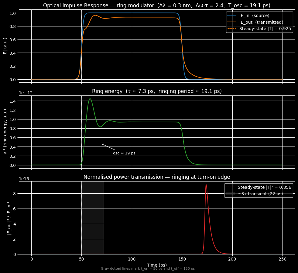
Simulated steady-state |T|: 0.925
Analytic  steady-state |T|: 0.925

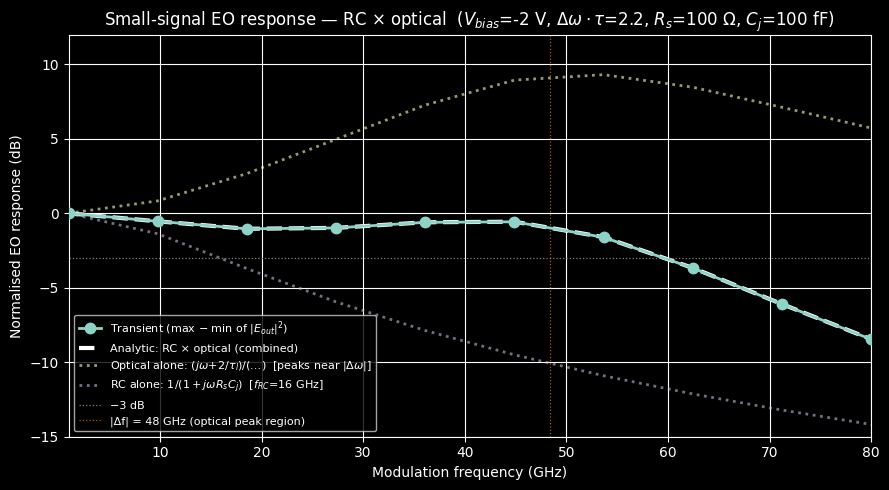
Small-signal electro-optic bandwidth

Note — time-domain is overkill here. A proper small-signal AC analysis or a Harmonic Balance (HB) solver would extract the EO frequency response in a single solve at each frequency, without integrating through many AC periods. circulax already has a Harmonic Balance solver and small-signal AC analysis is a planned feature. The purpose of this section is to verify that the time-domain DAE equations are equivalent to the analytic transfer function — i.e. the equations are correct — not to advocate transient simulation as the right tool for bandwidth characterisation in production.

A small sinusoidal voltage is applied to the ring modulator through an RC equivalent circuit that models a reverse-biased PN junction:

• R_s — series resistance (contact + waveguide)

• C_j — depletion capacitance (junction)

The combined small-signal EO response is limited by two first-order poles:

\[|H(f)| \propto \frac{1}{\sqrt{1 + (f/f_{\rm RC})^2}\;\sqrt{1 + (f/f_{\rm opt})^2}}\]

where \(f_{\rm RC} = 1/(2\pi R_s C_j)\) and \(f_{\rm opt} = 1/(2\pi\tau)\).

Simulation strategy: the DC operating point (optical CW + DC bias \(V_{\rm bias}\)) is found first and used as the initial condition at \(t = 0\). A small AC swing \(V_{\rm ac}\sin(2\pi f t)\) is then enabled at \(t = 10\,\text{ps}\). For each modulation frequency the output power amplitude (max \(-\) min of \(|E_{\rm out}|^2\)) is extracted from the last half of the simulation and normalised to the low-frequency value.

from circulax.components.electronic import Capacitor


@source(ports=("p1", "p2"), states=("i_src",))
def OpticalSourceStep(
    signals: Signals,
    s: States,
    t: float,
    power: float = 1.0,
    phase: float = 0.0,
) -> PhysicsReturn:
    """Constant-amplitude optical CW source (always on, no time dependence)."""
    amp = jnp.sqrt(power) * jnp.exp(1j * phase)
    constraint = (signals.p1 - signals.p2) - amp
    return {"p1": s.i_src, "p2": -s.i_src, "i_src": constraint}, {}


@source(ports=("p1", "p2"), states=("i_src",))
def BiasedACSource(
    signals: Signals,
    s: States,
    t: float,
    V_bias: float = -2.0,
    V_ac: float = 0.1,
    freq: float = 1e9,
    t_ac_start: float = 10e-12,
    rise_ac: float = 1e-12,
) -> PhysicsReturn:
    """DC-biased sinusoidal voltage source.

    Outputs V_bias (always present) plus V_ac * sin(2π * freq * t), with the
    AC component enabled smoothly at t_ac_start.  At t=0 the AC term is
    negligibly small (sigmoid(-10) ≈ 0), so solve_dc finds the correct DC
    operating point with only V_bias present.
    """
    v_ac = V_ac * jnp.sin(2.0 * jnp.pi * freq * t)
    ac_enable = jax.nn.sigmoid((t - t_ac_start) / rise_ac)
    v_total = V_bias + v_ac * ac_enable
    constraint = (signals.p1 - signals.p2) - v_total
    return {"p1": s.i_src, "p2": -s.i_src, "i_src": constraint}, {}


@component(ports=("p1", "p2", "v_e"), states=("a", "i_out"))
def RingModulatorEO(
    signals: Signals,
    s: States,
    ng: float = 3.8,
    L: float = 3.14159265e-5,
    gamma: float = 0.976,
    alpha0: float = 0.969,
    alpha1: float = 0.0,
    f_operating: float = 2.2904e14,
    f_resonance: float = 2.2901e14,
    v_to_wr: float = 0.0,
) -> PhysicsReturn:
    """Ring modulator with an external electrical voltage port ``v_e``.

    The voltage at port ``v_e`` modulates the ring resonance frequency via
    ``v_to_wr`` (rad/s/V).  The port is high-impedance: it draws no current
    (``F["v_e"] = 0``), so any driver circuit sees an open circuit.

    The physics is otherwise identical to :func:`RingModulator`, but ``voltage``
    is read from the external port rather than being a fixed parameter.
    """
    c = 2.998e8
    voltage = jnp.real(signals.v_e)  # electrical port — real part only

    tau_e = 2.0 * ng * L / ((1.0 - gamma**2) * c)
    alpha_v = alpha0 + alpha1 * voltage
    tau_l = 2.0 * ng * L / ((1.0 - alpha_v**2) * c)
    tau = 1.0 / (1.0 / tau_e + 1.0 / tau_l)
    coupling = jnp.sqrt(2.0 / tau_e)

    delta_omega = 2.0 * jnp.pi * (f_operating - f_resonance) + v_to_wr * voltage

    rhs_a = -1j * coupling * signals.p1 + 1j * delta_omega * s.a - s.a / tau
    E_o_expected = signals.p1 - 1j * coupling * s.a

    f = {
        "p1": 0.0 + 0.0j,
        "p2": s.i_out,
        "v_e": 0.0 + 0.0j,  # high-impedance electrical port
        "i_out": signals.p2 - E_o_expected,
        "a": -rhs_a,
    }
    q = {"a": s.a}
    return f, q

# ── Electrical RC parameters ──────────────────────────────────────────────
V_bias = -2.0  # V   — DC reverse bias (negative = reverse-biased PN junction)
V_ac = 0.2  # V   — small-signal swing (<<1, so response is linear)
R_s = 100.0  # Ω   — series resistance (contact + waveguide)
C_j = 100e-15  # F   — junction depletion capacitance
v_to_wr = 2.0 * np.pi * 2e9  # rad/s/V — EO coefficient (2 GHz/V resonance shift)
t_ac_start = 10e-12  # s   — delay before AC is enabled

f_RC = 1.0 / (2.0 * np.pi * R_s * C_j)  # electrical 3-dB bandwidth
f_opt_bw = 1.0 / (2.0 * np.pi * tau)  # optical photon-lifetime bandwidth

print(f"Electrical RC bandwidth : f_RC  = {f_RC / 1e9:.1f} GHz")
print(f"Optical photon-lifetime : f_opt = {f_opt_bw / 1e9:.1f} GHz")
print(f"EO coefficient          : dω/dV = {v_to_wr / (2e9 * np.pi):.1f} × 2π GHz/V")

# ── Models map ────────────────────────────────────────────────────────
models_map_ss = {
    "ground": lambda: 0,
    "optical_cw": OpticalSourceStep,
    "biased_ac": BiasedACSource,
    "ring_eo": RingModulatorEO,
    "resistor": Resistor,
    "capacitor": Capacitor,
}

# ── Netlist ───────────────────────────────────────────────────────────────────
# Topology:
#   OptSrc → Ring (optical path)
#   Vsrc → Rs → node_ve → Cj → GND  (electrical RC network)
#   Ring,v_e = node_ve  (high-impedance; ring reads voltage, draws no current)
net_dict_ss = {
    "instances": {
        "GND": {"component": "ground"},
        "OptSrc": {"component": "optical_cw", "settings": {"power": 1.0}},
        "Ring": {
            "component": "ring_eo",
            "settings": {
                "ng": ng,
                "L": L_ring,
                "gamma": gamma,
                "alpha0": alpha0,
                "f_operating": float(f_operating),
                "f_resonance": float(f_resonance),
                "v_to_wr": v_to_wr,
            },
        },
        "Load": {"component": "resistor", "settings": {"R": 1.0}},
        "Vsrc": {
            "component": "biased_ac",
            "settings": {
                "V_bias": V_bias,
                "V_ac": V_ac,
                "freq": 1e9,
                "t_ac_start": t_ac_start,
            },
        },
        "Rs": {"component": "resistor", "settings": {"R": R_s}},
        "Cj": {"component": "capacitor", "settings": {"C": C_j}},
    },
    "connections": {
        "GND,p1": ("OptSrc,p2", "Load,p2", "Vsrc,p2", "Cj,p2"),
        "OptSrc,p1": "Ring,p1",
        "Ring,p2": "Load,p1",
        "Vsrc,p1": "Rs,p1",
        "Rs,p2": ("Cj,p1", "Ring,v_e"),  # node_ve: RC junction & ring voltage port
    },
}

print("\nCompiling small-signal netlist...")
groups_ss, sys_size_ss, port_map_ss = compile_netlist(net_dict_ss, models_map_ss)

# ── DC operating point ────────────────────────────────────────────────────────────────
# At t=0: BiasedACSource outputs V_bias (AC term is sigmoid(-10) ≈ 0).
# OpticalSourceStep is always on.  solve_dc finds the joint optical + electrical
# steady state: ring at optical SS, node_ve = V_bias.
linear_strat_ss = analyze_circuit(groups_ss, sys_size_ss, is_complex=True)
y_guess_ss = jnp.zeros(sys_size_ss * 2, dtype=jnp.float64)
y0_ss = linear_strat_ss.solve_dc(groups_ss, y_guess_ss)

# Report DC state
ys0_complex = y0_ss[:sys_size_ss] + 1j * y0_ss[sys_size_ss:]
V_ve_dc = float(jnp.real(ys0_complex[port_map_ss["Ring,v_e"]]))
E_in_dc = ys0_complex[port_map_ss["Ring,p1"]]
E_out_dc = ys0_complex[port_map_ss["Ring,p2"]]
T_dc_sim = float(jnp.abs(E_out_dc) / (jnp.abs(E_in_dc) + 1e-20))

# Analytic DC transmission at the biased detuning
delta_omega_dc = 2.0 * np.pi * (f_operating - f_resonance) + v_to_wr * V_bias
x_dc = delta_omega_dc * tau
A_dc = 2.0 * tau / tau_e
T_dc_analytic = np.sqrt(((1 - A_dc) ** 2 + x_dc**2) / (1 + x_dc**2))

print(f"\nDC node_ve voltage : {V_ve_dc:.3f} V  (expected {V_bias:.1f} V)")
print(f"DC |T| simulated   : {T_dc_sim:.4f}")
print(f"DC |T| analytic    : {T_dc_analytic:.4f}")
print(f"DC Δω·τ            : {x_dc:.3f}")

Electrical RC bandwidth : f_RC  = 15.9 GHz
Optical photon-lifetime : f_opt = 21.7 GHz
EO coefficient          : dω/dV = 2.0 × 2π GHz/V

Compiling small-signal netlist...

DC node_ve voltage : -2.000 V  (expected -2.0 V)
DC |T| simulated   : 0.9142
DC |T| analytic    : 0.9142
DC Δω·τ            : 2.234

freqs_GHz = np.linspace(1.0, 80, 10)
N_periods = 10.0  # simulate this many AC periods per run
n_save = 500  # save this many points in the readout window
amplitudes = []  # will hold max(P_out) - min(P_out) per frequency

transient_sim_ss = setup_transient(groups=groups_ss, linear_strategy=linear_strat_ss)
E_out_node = port_map_ss["Ring,p2"]

print(f"Running {len(freqs_GHz)}-point frequency sweep …")
for idx, f_ghz in enumerate(freqs_GHz):
    f_hz = f_ghz * 1e9

    groups_f = update_group_params(groups_ss, "biased_ac", "freq", f_hz)

    t_sim = t_ac_start + N_periods / f_hz
    t_read = t_ac_start + (N_periods // 2) / f_hz
    ts_save = jnp.linspace(t_read, t_sim, n_save)

    dtmax = 1.0 / (20.0 * f_hz)  # ≥ 20 samples per AC period

    sol = transient_sim_ss(
        t0=0.0,
        t1=t_sim,
        dt0=min(1e-12, dtmax),
        y0=y0_ss,
        saveat=diffrax.SaveAt(ts=ts_save),
        max_steps=2_000_000,
        throw=False,
        args=(groups_f, sys_size_ss),
        stepsize_controller=diffrax.PIDController(rtol=1e-8, atol=1e-8, dtmax=dtmax),
    )

    if sol.result != diffrax.RESULTS.successful:
        print(
            f"  [{idx + 1:2d}/{len(freqs_GHz)}] {f_ghz:5.1f} GHz  WARNING: {sol.result}"
        )

    ys_c = sol.ys[:, :sys_size_ss] + 1j * sol.ys[:, sys_size_ss:]
    P_out = jnp.abs(ys_c[:, E_out_node]) ** 2
    P_norm = jnp.min(P_out[: int(-n_save / 2)])
    amplitudes.append(float(jnp.max(P_out[: int(-n_save / 2)]) - P_norm))

    if (idx + 1) % 2 == 0:
        print(f"  {idx + 1}/{len(freqs_GHz)} done")

print("Sweep complete.")

Running 10-point frequency sweep …

  2/10 done

  4/10 done

  6/10 done

  8/10 done

  10/10 done
Sweep complete.

omega_m = 2.0 * np.pi * freqs_GHz * 1e9  # rad/s

delta_omega_dc = (
    2.0 * np.pi * (float(f_operating) - float(f_resonance)) + v_to_wr * V_bias
)
inv_tau = 1.0 / tau
inv_tau_l = 1.0 / tau_l

# Electrical RC lowpass
H_RC = 1.0 / (1.0 + 1j * omega_m * R_s * C_j)

# Second-order optical transfer function
#   H_opt(jω) = (jω + 2/τ_l) / (Δω² + (1/τ)² − ω² + j(2/τ)ω)
denom_dc = delta_omega_dc**2 + inv_tau**2
H_opt = (1j * omega_m + 2.0 * inv_tau_l) / (
    -(omega_m**2) + 1j * 2.0 * inv_tau * omega_m + denom_dc
)

H_total = H_RC * H_opt
H_mag = np.abs(H_total)
H_norm = H_mag / H_mag[0]
H_dB = 20.0 * np.log10(H_norm)

H_RC_dB = 20.0 * np.log10(np.abs(H_RC) / np.abs(H_RC[0]))
H_opt_dB = 20.0 * np.log10(np.abs(H_opt) / np.abs(H_opt[0]))

f_pole_GHz = np.sqrt(delta_omega_dc**2 + inv_tau**2) / (2.0 * np.pi * 1e9)

amps = np.array(amplitudes)
amps_norm = amps / (amps[0])
amps_dB = 20.0 * np.log10(amps_norm)

print(
    f"DC-biased detuning  Δf      : {delta_omega_dc / (2 * np.pi * 1e9):.1f} GHz  (Δω·τ = {delta_omega_dc * tau:.2f})"
)
print(f"Optical pole magnitude      : {f_pole_GHz:.1f} GHz")
print(
    f"Optical peak (no RC)        : {float(np.max(H_opt_dB)):.1f} dB  at {freqs_GHz[np.argmax(H_opt_dB)]:.1f} GHz"
)
print(
    f"Combined peak (RC + optical): {float(np.max(H_dB)):.1f} dB  at {freqs_GHz[np.argmax(H_dB)]:.1f} GHz"
)

fig, ax = plt.subplots(figsize=(9, 5))

ax.plot(
    freqs_GHz,
    amps_dB,
    "o-",
    ms=7.5,
    linewidth=2.0,
    zorder=3,
    label="Transient (max − min of $|E_{out}|^2$)",
)
ax.plot(
    freqs_GHz, H_dB, "w--", linewidth=3.0, label="Analytic: RC × optical (combined)"
)
ax.plot(
    freqs_GHz,
    H_opt_dB,
    ":",
    linewidth=2.0,
    alpha=0.6,
    label=r"Optical alone: $(j\omega\!+\!2/\tau_l)/(…)$  [peaks near $|\Delta\omega|$]",
)
ax.plot(
    freqs_GHz,
    H_RC_dB,
    ":",
    linewidth=2.0,
    alpha=0.6,
    label=f"RC alone: $1/(1+j\\omega R_s C_j)$  [$f_{{RC}}$={f_RC / 1e9:.0f} GHz]",
)

ax.axhline(-3.0, color="gray", linestyle=":", linewidth=0.9, label="−3 dB")
ax.axvline(
    abs(delta_omega_dc) / (2 * np.pi * 1e9),
    color="tab:orange",
    linestyle=":",
    linewidth=0.9,
    alpha=0.7,
    label=f"|Δf| = {abs(delta_omega_dc) / (2 * np.pi * 1e9):.0f} GHz (optical peak region)",
)

ax.set_xlabel("Modulation frequency (GHz)")
ax.set_ylabel("Normalised EO response (dB)")
ax.set_title(
    f"Small-signal EO response — RC × optical  "
    f"($V_{{bias}}$={V_bias:.0f} V, $\\Delta\\omega\\cdot\\tau$={delta_omega_dc * tau:.1f}, "
    f"$R_s$={R_s:.0f} Ω, $C_j$={C_j * 1e15:.0f} fF)"
)
ax.set_xlim(freqs_GHz[0], freqs_GHz[-1])
ax.set_ylim(-15.0, 12.0)
ax.legend(fontsize=8, loc="lower left")
fig.tight_layout()
plt.show()

DC-biased detuning  Δf      : 48.4 GHz  (Δω·τ = 2.23)
Optical pole magnitude      : 53.1 GHz
Optical peak (no RC)        : 9.3 dB  at 53.7 GHz
Combined peak (RC + optical): 0.0 dB  at 1.0 GHz

---

Part 3: EO Bandwidth via Harmonic Balance

The transient sweep above runs 25 independent simulations — one per frequency. Harmonic Balance (HB) finds the periodic steady state directly, without time-stepping to steady state, and jax.vmap solves all frequencies in a single XLA compilation.

The modulation frequency \(f_m\) is the HB fundamental. With \(N_h = 5\) harmonics (\(K = 11\) time samples per period) the Newton loop converges in ~20 iterations independent of \(f_m\).

How the sweep works

def hb_sweep_point(freq):             # freq is now a JAX argument — vmappable
    run_hb = setup_harmonic_balance(groups_hb, num_vars_hb,
                                    freq=freq, num_harmonics=N_harm_hb,
                                    is_complex=True)   # photonic circuit
    y_time, _ = run_hb(y_dc_hb)
    E_out = y_time[:, vout_hb] + 1j * y_time[:, vout_hb + num_vars_hb]
    P_out = jnp.abs(E_out) ** 2
    return jnp.max(P_out) - jnp.min(P_out)

amps_hb = jax.jit(jax.vmap(hb_sweep_point))(sweep_freqs)

is_complex=True tells the HB solver to use the unrolled [re | im] block representation that photonic circuits require.

from circulax import setup_harmonic_balance


@source(ports=("p1", "p2"), states=("i_src",))
def BiasedSinSource(
    signals: Signals,
    s: States,
    t: float,
    V_bias: float = -2.0,
    V_ac: float = 0.1,
    freq: float = 1e9,
) -> PhysicsReturn:
    """DC-biased sinusoidal source, exactly periodic at ``freq``.

    At t = 0: V = V_bias (no AC), giving the same DC operating point as
    :class:`BiasedACSource` with the AC component disabled.
    """
    v = V_bias + V_ac * jnp.sin(2.0 * jnp.pi * freq * t)
    return {"p1": s.i_src, "p2": -s.i_src, "i_src": (signals.p1 - signals.p2) - v}, {}


models_map_hb = {
    "ground": lambda: 0,
    "optical_cw": OpticalSourceStep,
    "biased_sin": BiasedSinSource,
    "ring_eo": RingModulatorEO,
    "resistor": Resistor,
    "capacitor": Capacitor,
}

net_dict_hb = {
    "instances": {
        "GND": {"component": "ground"},
        "OptSrc": {"component": "optical_cw", "settings": {"power": 1.0}},
        "Ring": {
            "component": "ring_eo",
            "settings": {
                "ng": ng,
                "L": L_ring,
                "gamma": gamma,
                "alpha0": alpha0,
                "f_operating": float(f_operating),
                "f_resonance": float(f_resonance),
                "v_to_wr": v_to_wr,
            },
        },
        "Load": {"component": "resistor", "settings": {"R": 1.0}},
        "Vsrc": {
            "component": "biased_sin",
            "settings": {
                "V_bias": V_bias,
                "V_ac": V_ac,
                "freq": 1e9,  # placeholder; updated per sweep point
            },
        },
        "Rs": {"component": "resistor", "settings": {"R": R_s}},
        "Cj": {"component": "capacitor", "settings": {"C": C_j}},
    },
    "connections": {
        "GND,p1": ("OptSrc,p2", "Load,p2", "Vsrc,p2", "Cj,p2"),
        "OptSrc,p1": "Ring,p1",
        "Ring,p2": "Load,p1",
        "Vsrc,p1": "Rs,p1",
        "Rs,p2": ("Cj,p1", "Ring,v_e"),
    },
}

print("Compiling HB netlist...")
groups_hb, num_vars_hb, port_map_hb = compile_netlist(net_dict_hb, models_map_hb)

linear_strat_hb = analyze_circuit(groups_hb, num_vars_hb, is_complex=True)
y_dc_hb = linear_strat_hb.solve_dc(
    groups_hb, jnp.zeros(num_vars_hb * 2, dtype=jnp.float64)
)

ys0_hb = y_dc_hb[:num_vars_hb] + 1j * y_dc_hb[num_vars_hb:]
E_in_dc_hb = ys0_hb[port_map_hb["Ring,p1"]]
E_out_dc_hb = ys0_hb[port_map_hb["Ring,p2"]]
T_dc_hb = float(jnp.abs(E_out_dc_hb) / (jnp.abs(E_in_dc_hb) + 1e-20))
print(f"\nDC |T| (HB netlist) : {T_dc_hb:.4f}  (transient: {T_dc_sim:.4f})")

Compiling HB netlist...

DC |T| (HB netlist) : 0.9142  (transient: 0.9142)

N_harm_hb = 5  # 5 harmonics → K = 11 time samples per period
K_hb = 2 * N_harm_hb + 1
f_demo = 1e9  # 1 GHz single-point demo

groups_hb_demo = update_group_params(groups_hb, "biased_sin", "freq", f_demo)

run_hb_demo = setup_harmonic_balance(
    groups_hb_demo, num_vars_hb, freq=f_demo, num_harmonics=N_harm_hb, is_complex=True
)
y_time_demo, _ = run_hb_demo(y_dc_hb)
print(f"HB converged at {f_demo / 1e9:.0f} GHz.  y_time shape: {y_time_demo.shape}")

# Reconstruct complex optical fields from the unrolled [re | im] state.
vout_hb = port_map_hb["Ring,p2"]
vin_hb = port_map_hb["Ring,p1"]
T_period_demo = 1.0 / f_demo
t_hb_demo = np.linspace(0, T_period_demo * 1e9, K_hb, endpoint=False)  # ns

E_in_demo = y_time_demo[:, vin_hb] + 1j * y_time_demo[:, vin_hb + num_vars_hb]
E_out_demo = y_time_demo[:, vout_hb] + 1j * y_time_demo[:, vout_hb + num_vars_hb]
P_in_demo = jnp.abs(E_in_demo) ** 2
P_out_demo = jnp.abs(E_out_demo) ** 2

fig, ax = plt.subplots(figsize=(8, 3.5))
ax.plot(
    t_hb_demo, np.array(P_in_demo), "C0o-", ms=7, label=r"$|E_\mathrm{in}|^2$  (CW)"
)
ax.plot(
    t_hb_demo,
    np.array(P_out_demo),
    "C1s-",
    ms=7,
    label=r"$|E_\mathrm{out}|^2$  (modulated)",
)
ax.axhline(
    T_dc_hb**2, color="C1", ls="--", lw=0.8, label=f"DC $|T|^2 = {T_dc_hb**2:.3f}$"
)
ax.set_xlabel("Time (ns)")
ax.set_ylabel("Power (a.u.)")
ax.set_title(
    f"HB waveform at $f_m$ = {f_demo / 1e9:.0f} GHz  "
    f"($K$ = {K_hb} points, $N_h$ = {N_harm_hb})"
)
ax.legend()
plt.tight_layout()
plt.show()

amp_demo = float(jnp.max(P_out_demo) - jnp.min(P_out_demo))
print(f"P_out oscillation amplitude: {amp_demo:.4e} W  (peak-to-peak power modulation)")

HB converged at 1 GHz.  y_time shape: (11, 18)

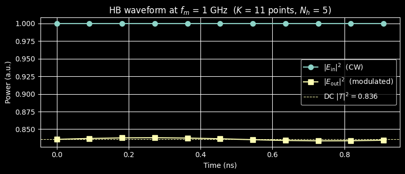
P_out oscillation amplitude: 4.4694e-03 W  (peak-to-peak power modulation)

def hb_sweep_point(freq):
    """HB solve at one modulation frequency — vmappable over freq."""
    g_f = update_group_params(groups_hb, "biased_sin", "freq", freq)

    run_hb = setup_harmonic_balance(
        g_f, num_vars_hb, freq=freq, num_harmonics=N_harm_hb, is_complex=True
    )
    y_time, _ = run_hb(y_dc_hb)

    E_out = y_time[:, vout_hb] + 1j * y_time[:, vout_hb + num_vars_hb]
    P_out = jnp.abs(E_out) ** 2
    return jnp.max(P_out) - jnp.min(P_out)


freqs_GHz_HB = jnp.array(
    freqs_GHz - 0.5 * jnp.diff(freqs_GHz)[0]
)  # offsetting only for visualization
sweep_freqs_hb = freqs_GHz_HB * 1e9

print(f"Running vmapped HB sweep over {len(sweep_freqs_hb)} frequencies (1–50 GHz)...")
amps_hb = jax.jit(jax.vmap(hb_sweep_point))(sweep_freqs_hb)
print("Done.")

amps_hb_np = np.array(amps_hb)
amps_hb_norm = amps_hb_np / (amps_hb_np[0] + 1e-30)
amps_hb_dB = 20.0 * np.log10(amps_hb_norm + 1e-30)

fig, ax = plt.subplots(figsize=(9, 5))

ax.plot(
    freqs_GHz,
    amps_dB,
    "o-",
    ms=7.5,
    linewidth=2.0,
    zorder=3,
    label="Transient",
)
ax.plot(
    freqs_GHz_HB,
    amps_hb_dB,
    "D--",
    ms=5,
    linewidth=1.5,
    zorder=4,
    label=f"HB vmap ({len(sweep_freqs_hb)} freqs, one XLA call, $N_h$={N_harm_hb})",
)
ax.plot(freqs_GHz, H_dB, "w-", linewidth=2.0, alpha=0.7, label="Analytic: RC × optical")
ax.plot(
    freqs_GHz,
    H_opt_dB,
    ":",
    linewidth=2.0,
    alpha=0.5,
    label=r"Optical alone: $(j\omega + 2/\tau_l)/(…)$",
)
ax.plot(
    freqs_GHz,
    H_RC_dB,
    ":",
    linewidth=2.0,
    alpha=0.5,
    label=f"RC alone  [$f_{{RC}}$ = {f_RC / 1e9:.0f} GHz]",
)

ax.axhline(-3.0, color="gray", linestyle=":", linewidth=1.5, label="−3 dB")
ax.axvline(
    abs(delta_omega_dc) / (2 * np.pi * 1e9),
    color="tab:orange",
    linestyle=":",
    linewidth=0.9,
    alpha=0.7,
    label=f"|Δf| = {abs(delta_omega_dc) / (2 * np.pi * 1e9):.0f} GHz",
)

ax.set_xlabel("Modulation frequency (GHz)")
ax.set_ylabel("Normalised EO response (dB)")
ax.set_title(
    f"EO bandwidth — HB vmap vs transient vs analytic  "
    f"($V_{{bias}}$={V_bias:.0f} V, $\\Delta\\omega\\cdot\\tau$={delta_omega_dc * tau:.1f})"
)
ax.set_xlim(freqs_GHz[0], freqs_GHz[-1])
ax.set_ylim(-15.0, 12.0)
ax.legend(fontsize=8, loc="lower left")
fig.tight_layout()
plt.show()

print("\nFreq (GHz)  | Transient (dB) | HB vmap (dB) | Analytic (dB)")
print("-" * 60)
for f, a_tr, a_hb, a_an in zip(
    freqs_GHz[::5], amps_dB[::5], amps_hb_dB[::5], H_dB[::5]
):
    print(
        f"  {f:5.1f}       |   {a_tr:+6.2f}        |  {a_hb:+6.2f}       | {a_an:+6.2f}"
    )

Running vmapped HB sweep over 10 frequencies (1–50 GHz)...

Done.

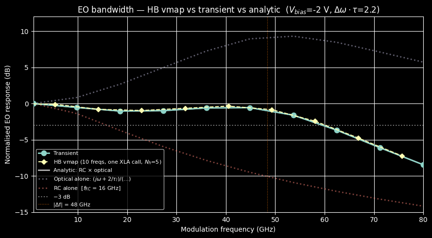
Freq (GHz)  | Transient (dB) | HB vmap (dB) | Analytic (dB)
------------------------------------------------------------
    1.0       |    +0.00        |   +0.00       |  +0.00
   44.9       |    -0.57        |   -0.35       |  -0.56

---

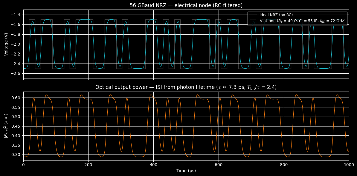
Part 4: Large-Signal NRZ Eye Diagram

The small-signal frequency response in Part 3 characterises the ring modulator’s linear bandwidth, but it cannot predict the actual eye opening under large-signal digital modulation. Three physical effects cause eye closure and distortion that the frequency response alone cannot capture:

1. Photon lifetime ISI: The ring energy \(a(t)\) decays with time constant \(\tau \approx 7.3\,\text{ps}\), comparable to the 56 GBaud bit period \(T_{\rm bit} \approx 17.9\,\text{ps}\) (ratio \(T_{\rm bit}/\tau \approx 2.4\)). Consecutive bits see different initial ring states — a “1” after many “0”s opens differently from a “1” after many “1”s. The electrical RC bandwidth is set to \(f_{\rm RC} \approx 72\,\text{GHz} \gg f_{\rm opt} \approx 22\,\text{GHz}\) so the photon lifetime is the sole bandwidth-limiting mechanism.

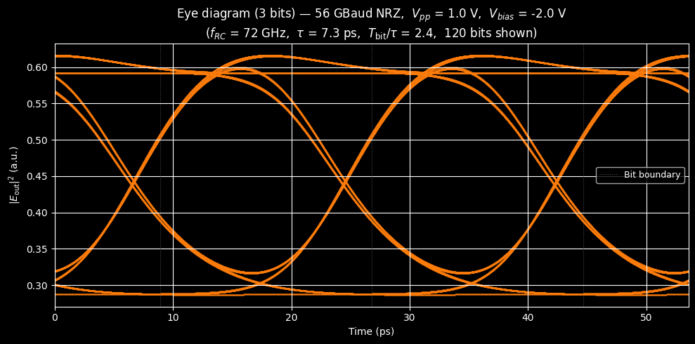
2. Nonlinear Lorentzian transfer function: The ring is biased at \(\Delta\omega\cdot\tau = 1\) (on the steepest slope of the resonance), giving a large extinction ratio for a \(V_{\rm pp} = 1\,\text{V}\) swing. Even so, positive and negative half-swings produce asymmetric optical excursions because the Lorentzian is nonlinear.

3. Voltage-dependent loss (eye tilt): A small voltage-dependent round-trip amplitude \(\alpha_1 = 0.007\,\text{V}^{-1}\) makes the ring photon lifetime slightly longer at \(V_{\rm high}\) (less loss) than at \(V_{\rm low}\) (more loss). This asymmetric ISI creates a characteristic tilt in the upper and lower eye rails.

The NRZ source is modelled as a sum of sigmoid transitions — fully JAX-compatible (jittable and vmappable) — driven by a 128-bit PRBS-like pattern.

@source(ports=("p1", "p2"), states=("i_src",))
def NRZSource(
    signals: Signals,
    s: States,
    t: float,
    V_low: float = -2.5,
    V_high: float = -1.5,
    T_bit: float = 1 / 56e9,
    rise: float = 2e-12,
    bits=(0.0,) * 32,  # tuple default (hashable); pass jnp.array in practice
    t_start: float = 0.0,
) -> PhysicsReturn:
    """NRZ voltage source driven by a fixed bit pattern.

    Voltage is a sum of sigmoid step functions at each bit transition.
    ``bits`` is an array of 0/1 values.  At t < t_start the output is V_low
    (all sigmoids ≈ 0), so solve_dc called at t=0 finds the correct DC
    operating point when t_start > 0.
    """
    bits_arr = jnp.asarray(bits)
    prev = jnp.concatenate([jnp.zeros(1), bits_arr[:-1]])
    delta_bits = bits_arr - prev
    bit_times = jnp.arange(len(bits_arr)) * T_bit + t_start
    v_norm = jnp.sum(delta_bits * jax.nn.sigmoid((t - bit_times) / rise))
    v = V_low + (V_high - V_low) * v_norm
    constraint = (signals.p1 - signals.p2) - v
    return {"p1": s.i_src, "p2": -s.i_src, "i_src": constraint}, {}


# ── NRZ signal parameters ──────────────────────────────────────────────────────
T_bit_nrz = 1.0 / 56e9  # ≈ 17.86 ps per bit
N_bits_nrz = 128  # 128-bit pattern
rise_nrz = 2e-12  # 2 ps rise time (≈ 11 % of T_bit)
t_start_nrz = T_bit_nrz  # quiet preamble: ring settles at V_low before first bit

V_bias = -2.0
V_pp = 1.0
V_low_nrz = V_bias - 0.5 * V_pp
V_high_nrz = V_bias + 0.5 * V_pp

# 32-bit PRBS-like pattern tiled 4× for 128 bits
_bits32 = jnp.array(
    [
        1,
        0,
        1,
        1,
        0,
        0,
        1,
        0,
        1,
        1,
        1,
        0,
        0,
        1,
        1,
        0,
        1,
        0,
        0,
        0,
        1,
        1,
        0,
        1,
        0,
        1,
        0,
        0,
        1,
        1,
        1,
        0,
    ],
    dtype=jnp.float64,
)
bits_nrz = jnp.tile(_bits32, 4)  # shape (128,)

t_end_nrz = t_start_nrz + N_bits_nrz * T_bit_nrz  # ≈ 2.3 ns total

# Voltage-dependent internal loss: alpha_v = alpha0 + alpha1_eo * V
# With reverse-bias convention (negative voltages), alpha1_eo > 0 means
# more reverse bias (more negative V) → lower alpha_v → more internal loss.
# Ring stays over-coupled (alpha_v < gamma) throughout the drive range.
alpha1_eo = 0.007  # V⁻¹  (positive; negative drive voltages give less loss at V_high)

# ── Eye-diagram circuit parameters (eye section only) ─────────────────────────
# f_RC >> f_opt so the photon lifetime is the sole bandwidth bottleneck.
R_s_eye = 40.0  # Ω   (low contact + driver resistance)
C_j_eye = 55e-15  # F   (compact depletion capacitance)
f_RC_eye = 1.0 / (2.0 * np.pi * R_s_eye * C_j_eye)
# Realistic EO coefficient for silicon PN ring at 1310 nm: ~15 GHz/V resonance shift
v_to_wr_eye = 2.0 * np.pi * 15e9  # rad/s/V

# Bias at Δω·τ = 1 (steepest slope of Lorentzian → maximum modulation depth)
# Solving 2π(f_op − f_res_eye) + v_to_wr_eye × V_bias = 1/τ for f_res_eye:
V_bias_nrz = (V_low_nrz + V_high_nrz) / 2.0  # = −2 V
detuning_eye_hz = (1.0 / tau - v_to_wr_eye * V_bias_nrz) / (2.0 * np.pi)
f_resonance_eye = float(f_operating - detuning_eye_hz)

f_opt_eye = 1.0 / (2.0 * np.pi * tau)
print(
    f"56 GBaud NRZ: T_bit = {T_bit_nrz * 1e12:.2f} ps,  τ = {tau * 1e12:.2f} ps  (T_bit/τ = {T_bit_nrz / tau:.1f})"
)
print(
    f"Optical bandwidth: f_opt = {f_opt_eye / 1e9:.1f} GHz  |  f_RC = {f_RC_eye / 1e9:.0f} GHz  (optically limited)"
)
print(
    f"Bias detuning: Δω·τ = 1.00 at V_bias = {V_bias_nrz:.1f} V  (f_res_eye = f_op − {detuning_eye_hz / 1e9:.1f} GHz)"
)
print(f"Simulation: {N_bits_nrz} bits, t_end = {t_end_nrz * 1e12:.0f} ps")
# Transmission and τ_l at each NRZ level
for _V, _label in [(V_low_nrz, "V_low"), (V_high_nrz, "V_high")]:
    _av = alpha0 + alpha1_eo * _V
    _tl = 2.0 * ng * L_ring / ((1.0 - _av**2) * 2.998e8)
    _dw = 2.0 * np.pi * detuning_eye_hz + v_to_wr_eye * _V
    _x = _dw * tau
    _A = 2.0 * tau / tau_e
    _T = np.sqrt(((1 - _A) ** 2 + _x**2) / (1 + _x**2))
    print(
        f"  {_label}={_V}V: α_v={_av:.4f}, τ_l={_tl * 1e12:.1f} ps, Δω·τ={_x:.2f}, |T|={_T:.3f}"
    )

# ── Models and netlist ─────────────────────────────────────────────────────────
models_map_eye = {
    "ground": lambda: 0,
    "optical_cw": OpticalSourceStep,
    "nrz_src": NRZSource,
    "ring_eo": RingModulatorEO,
    "resistor": Resistor,
    "capacitor": Capacitor,
}

net_dict_eye = {
    "instances": {
        "GND": {"component": "ground"},
        "OptSrc": {"component": "optical_cw", "settings": {"power": 1.0}},
        "Ring": {
            "component": "ring_eo",
            "settings": {
                "ng": ng,
                "L": L_ring,
                "gamma": gamma,
                "alpha0": alpha0,
                "alpha1": alpha1_eo,  # voltage-dependent internal loss (eye diagram only)
                "f_operating": float(f_operating),
                "f_resonance": float(f_resonance_eye),
                "v_to_wr": v_to_wr_eye,
            },
        },
        "Load": {"component": "resistor", "settings": {"R": 1.0}},
        "Vsrc": {
            "component": "nrz_src",
            "settings": {
                "V_low": V_low_nrz,
                "V_high": V_high_nrz,
                "T_bit": T_bit_nrz,
                "rise": rise_nrz,
                "bits": bits_nrz,
                "t_start": t_start_nrz,
            },
        },
        "Rs": {"component": "resistor", "settings": {"R": R_s_eye}},
        "Cj": {"component": "capacitor", "settings": {"C": C_j_eye}},
    },
    "connections": {
        "GND,p1": ("OptSrc,p2", "Load,p2", "Vsrc,p2", "Cj,p2"),
        "OptSrc,p1": "Ring,p1",
        "Ring,p2": "Load,p1",
        "Vsrc,p1": "Rs,p1",
        "Rs,p2": ("Cj,p1", "Ring,v_e"),
    },
}

print("\nCompiling NRZ netlist...")
groups_eye, sys_size_eye, port_map_eye = compile_netlist(net_dict_eye, models_map_eye)

# DC at t=0: NRZSource outputs V_low (all sigmoids ≈ 0, since t_start = T_bit >> rise)
linear_strat_eye = analyze_circuit(groups_eye, sys_size_eye, is_complex=True)
y0_nrz = linear_strat_eye.solve_dc(
    groups_eye, jnp.zeros(sys_size_eye * 2, dtype=jnp.float64)
)

ys0_eye = y0_nrz[:sys_size_eye] + 1j * y0_nrz[sys_size_eye:]
V_ve0 = float(jnp.real(ys0_eye[port_map_eye["Ring,v_e"]]))
T_dc_eye = float(
    jnp.abs(ys0_eye[port_map_eye["Ring,p2"]])
    / (jnp.abs(ys0_eye[port_map_eye["Ring,p1"]]) + 1e-20)
)
print(f"DC: V_ve = {V_ve0:.3f} V  (expected {V_low_nrz:.1f} V),  |T| = {T_dc_eye:.4f}")

56 GBaud NRZ: T_bit = 17.86 ps,  τ = 7.34 ps  (T_bit/τ = 2.4)
Optical bandwidth: f_opt = 21.7 GHz  |  f_RC = 72 GHz  (optically limited)
Bias detuning: Δω·τ = 1.00 at V_bias = -2.0 V  (f_res_eye = f_op − 51.7 GHz)
Simulation: 128 bits, t_end = 2304 ps
  V_low=-2.5V: α_v=0.9515, τ_l=8.4 ps, Δω·τ=0.65, |T|=0.557
  V_high=-1.5V: α_v=0.9585, τ_l=9.8 ps, Δω·τ=1.35, |T|=0.806

Compiling NRZ netlist...

DC: V_ve = -2.500 V  (expected -2.5 V),  |T| = 0.5367

transient_sim_nrz = setup_transient(groups=groups_eye, linear_strategy=linear_strat_eye)

controller_nrz = diffrax.PIDController(
    rtol=1e-6,
    atol=1e-8,
    dtmax=rise_nrz / 2,  # ≤ 1 ps per step — resolves each sigmoid transition
)

print(
    f"Running NRZ transient simulation ({N_bits_nrz} bits at 56 GBaud, t_end = {t_end_nrz * 1e12:.0f} ps)…"
)
sol_nrz = transient_sim_nrz(
    t0=0.0,
    t1=t_end_nrz,
    dt0=1e-13,
    y0=y0_nrz,
    saveat=diffrax.SaveAt(ts=jnp.linspace(0.0, t_end_nrz, 32000)),
    max_steps=8_000_000,
    throw=False,
    stepsize_controller=controller_nrz,
)

if sol_nrz.result == diffrax.RESULTS.successful:
    print("Simulation successful")
else:
    print(f"Simulation ended with: {sol_nrz.result}")

ys_complex_nrz = sol_nrz.ys[:, :sys_size_eye] + 1j * sol_nrz.ys[:, sys_size_eye:]
ts_ps_nrz = sol_nrz.ts * 1e12

Running NRZ transient simulation (128 bits at 56 GBaud, t_end = 2304 ps)…

Simulation successful

def fold_eye(P_out, ts, t_start, T_bit, N_skip=8):
    """Fold optical power into a 3-period eye diagram, auto-centred on the crossing."""
    t_eye_start = t_start + N_skip * T_bit
    mask = ts >= t_eye_start
    T_ps = T_bit * 1e12
    P = np.array(P_out[mask])
    t_raw = np.array((ts[mask] - t_eye_start) % T_bit) * 1e12
    n_bins = 200
    edges = np.linspace(0, T_ps, n_bins + 1)
    ctrs = (edges[:-1] + edges[1:]) / 2
    bidx = np.clip(np.digitize(t_raw, edges) - 1, 0, n_bins - 1)
    means = np.array(
        [P[bidx == i].mean() if np.any(bidx == i) else np.nan for i in range(n_bins)]
    )
    P_mid = (np.nanmax(means) + np.nanmin(means)) / 2
    cross_ps = ctrs[np.nanargmin(np.abs(means - P_mid))]
    phase = T_bit / 2 - cross_ps * 1e-12
    t_fold = np.array(((ts[mask] - t_eye_start + phase) % T_bit) * 1e12)
    t3 = np.concatenate([t_fold, t_fold + T_ps, t_fold + 2 * T_ps])
    P3 = np.concatenate([P, P, P])
    return t3, P3, T_ps


V_ve_nrz = jnp.real(ys_complex_nrz[:, port_map_eye["Ring,v_e"]])
E_out_nrz = ys_complex_nrz[:, port_map_eye["Ring,p2"]]
P_out_nrz = jnp.abs(E_out_nrz) ** 2

t_plot_end_ps = 1000.0
t_mask = ts_ps_nrz <= t_plot_end_ps

fig, axes = plt.subplots(2, 1, figsize=(12, 6), sharex=True)

transitions_ps = (t_start_nrz + np.arange(N_bits_nrz) * T_bit_nrz) * 1e12
levels_V = V_low_nrz + (V_high_nrz - V_low_nrz) * np.array(bits_nrz)
edges_ps = np.concatenate([[0.0], transitions_ps, [t_end_nrz * 1e12]])
values_V = np.concatenate([[V_low_nrz], levels_V])

axes[0].stairs(
    values_V,
    edges_ps,
    color="gray",
    alpha=0.5,
    linewidth=1.0,
    label="Ideal NRZ (no RC)",
)
axes[0].plot(
    ts_ps_nrz[t_mask],
    np.array(V_ve_nrz[t_mask]),
    color="tab:cyan",
    linewidth=0.8,
    label=f"V at ring ($R_s$ = {R_s_eye:.0f} Ω, $C_j$ = {C_j_eye * 1e15:.0f} fF, $f_{{RC}}$ = {f_RC_eye / 1e9:.0f} GHz)",
)
axes[0].set_ylabel("Voltage (V)")
axes[0].set_title("56 GBaud NRZ — electrical node (RC-filtered)")
axes[0].legend(loc="upper right", fontsize=9)
axes[0].set_ylim(V_low_nrz - 0.2, V_high_nrz + 0.2)
axes[0].set_xlim(0, t_plot_end_ps)

axes[1].plot(
    ts_ps_nrz[t_mask], np.array(P_out_nrz[t_mask]), color="tab:orange", linewidth=0.8
)
axes[1].set_ylabel(r"$|E_\mathrm{out}|^2$ (a.u.)")
axes[1].set_xlabel("Time (ps)")
axes[1].set_title(
    r"Optical output power — ISI from photon lifetime ($\tau \approx$ "
    + f"{tau * 1e12:.1f} ps, $T_{{\\rm bit}}/\\tau$ = {T_bit_nrz / tau:.1f})"
)
fig.tight_layout()
plt.show()

# ── Eye diagram (3 bits wide, auto-centred on optical crossing) ──────────────────────
t3_nrz, P3_nrz, T_ps_nrz = fold_eye(
    P_out_nrz, sol_nrz.ts, t_start_nrz, T_bit_nrz, N_skip=8
)

fig, ax = plt.subplots(figsize=(10, 5))
ax.scatter(t3_nrz, P3_nrz, s=0.5, alpha=0.3, rasterized=True, color="tab:orange")
ax.set_xlabel("Time (ps)")
ax.set_ylabel(r"$|E_\mathrm{out}|^2$ (a.u.)")
ax.set_xlim(0, 3 * T_ps_nrz)
for k in range(3):
    ax.axvline(
        (k + 0.5) * T_ps_nrz,
        color="gray",
        linestyle=":",
        linewidth=0.8,
        alpha=0.6,
        label="Bit boundary" if k == 0 else None,
    )
ax.set_title(
    f"Eye diagram (3 bits) — 56 GBaud NRZ,  $V_{{pp}}$ = {V_high_nrz - V_low_nrz:.1f} V,  "
    f"$V_{{bias}}$ = {(V_low_nrz + V_high_nrz) / 2:.1f} V\n"
    f"($f_{{RC}}$ = {f_RC_eye / 1e9:.0f} GHz,  $\\tau$ = {tau * 1e12:.1f} ps,  "
    f"$T_{{\\rm bit}}/\\tau$ = {T_bit_nrz / tau:.1f},  {N_bits_nrz - 8} bits shown)"
)
ax.legend(fontsize=9)
fig.tight_layout()
plt.show()

---

Part 5: V_bias Sweep via jax.vmap

With jax.vmap, we can run eye diagram simulations for multiple bias voltages in a single JIT-compiled XLA call — analogous to the HB frequency sweep in Part 3.

Each sweep point updates the NRZ voltage levels and ring resonance frequency (to keep \(\Delta\omega\cdot\tau = 1\) at the new bias), then runs the full transient simulation. The DC initial conditions are pre-computed in a Python loop.

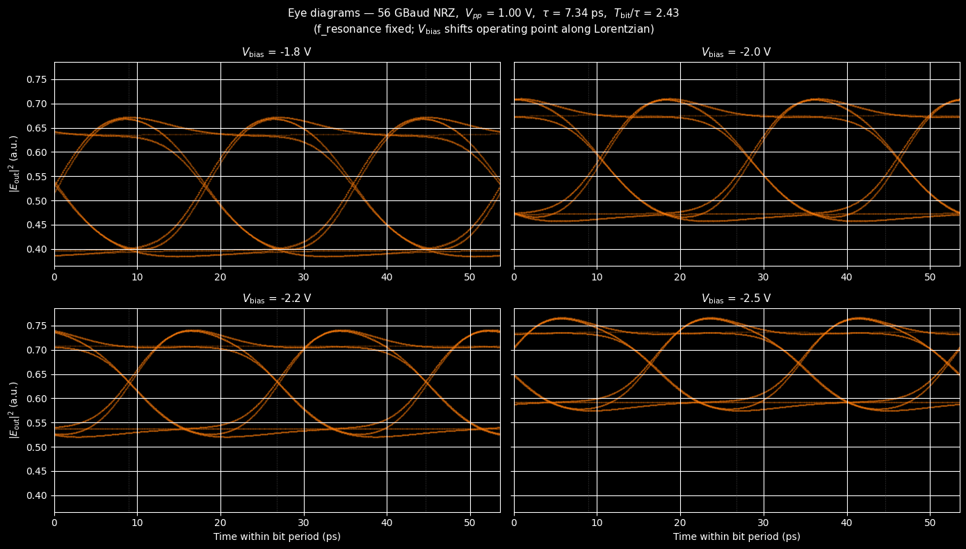
The four panels below show how the eye diagram changes as \(V_\text{bias}\) shifts the operating point along the ring Lorentzian:

• Less negative bias → ring further from resonance → higher mean transmission, wider eye

• More negative bias → ring closer to resonance → deeper modulation, stronger nonlinear ISI

# Pre-compute DC initial conditions for each V_bias (one Newton solve per point). This is cheap
V_bias_sweep = jnp.array([-1.75, -2.0, -2.25, -2.5])

y0_sweep = []
for Vb in V_bias_sweep:
    Vb = float(Vb)
    g = update_group_params(groups_eye, "nrz_src", "V_low", Vb - 0.5 * V_pp)
    g = update_group_params(g, "nrz_src", "V_high", Vb + 0.5 * V_pp)
    g = update_group_params(g, "ring_eo", "f_resonance", f_operating)
    y0_sweep.append(
        linear_strat_eye.solve_dc(g, jnp.zeros(sys_size_eye * 2, dtype=jnp.float64))
    )
y0_sweep = jnp.stack(y0_sweep)  # shape (4, sys_size_eye * 2)

N_bits_vmap = 32  # 32 bits keeps per-sweep memory small
t_end_vmap = t_start_nrz + N_bits_vmap * T_bit_nrz  # ≈ 589 ps (vs 2.3 ns for Part 4)
ts_save_vmap = jnp.linspace(0.0, t_end_vmap, 4000)


def run_eye_for_vbias(V_bias_val, y0):
    """Single transient eye-diagram run, parameterised by V_bias — vmappable."""
    V_low_val = V_bias_val - 0.5 * V_pp
    V_high_val = V_bias_val + 0.5 * V_pp
    g = update_group_params(groups_eye, "nrz_src", "V_low", V_low_val)
    g = update_group_params(g, "nrz_src", "V_high", V_high_val)
    g = update_group_params(g, "ring_eo", "f_resonance", f_operating)

    sim = setup_transient(groups=g, linear_strategy=linear_strat_eye)
    sol = sim(
        t0=0.0,
        t1=t_end_vmap,
        dt0=1e-13,
        y0=y0,
        saveat=diffrax.SaveAt(ts=ts_save_vmap),
        max_steps=8_000_000,
        throw=False,
        stepsize_controller=diffrax.PIDController(
            rtol=1e-6, atol=1e-8, dtmax=rise_nrz / 2
        ),
    )
    ys = sol.ys[:, :sys_size_eye] + 1j * sol.ys[:, sys_size_eye:]
    return jnp.abs(ys[:, port_map_eye["Ring,p2"]]) ** 2


print(
    f"Running jax.vmap over {len(V_bias_sweep)} V_bias values: {V_bias_sweep.tolist()} V"
)
P_out_sweep = jax.jit(jax.vmap(run_eye_for_vbias))(V_bias_sweep, y0_sweep)
print(
    f"Done.  Output shape: {P_out_sweep.shape}  ({P_out_sweep.shape[0]} sweeps \u00d7 {P_out_sweep.shape[1]} time points)"
)

Running jax.vmap over 4 V_bias values: [-1.75, -2.0, -2.25, -2.5] V

Done.  Output shape: (4, 4000)  (4 sweeps × 4000 time points)

fig, axes = plt.subplots(2, 2, figsize=(14, 8), sharey=True)
axes_flat = axes.flatten()

for idx, Vb in enumerate(V_bias_sweep):
    ax = axes_flat[idx]
    t3, P3, T_ps = fold_eye(
        P_out_sweep[idx], ts_save_vmap, t_start_nrz, T_bit_nrz, N_skip=4
    )
    ax.scatter(t3, P3, s=0.3, alpha=0.25, rasterized=True, color="tab:orange")
    ax.set_xlim(0, 3 * T_ps)
    for k in range(3):
        ax.axvline(
            (k + 0.5) * T_ps, color="gray", linestyle=":", linewidth=0.7, alpha=0.5
        )
    ax.set_title(f"$V_\\mathrm{{bias}}$ = {float(Vb):.1f} V", fontsize=11)
    if idx >= 2:
        ax.set_xlabel("Time within bit period (ps)")
    if idx % 2 == 0:
        ax.set_ylabel(r"$|E_\mathrm{out}|^2$ (a.u.)")

fig.suptitle(
    f"Eye diagrams — 56 GBaud NRZ,  $V_{{pp}}$ = {V_pp:.2f} V,  "
    f"$\\tau$ = {tau * 1e12:.2f} ps,  $T_\\mathrm{{bit}}/\\tau$ = {T_bit_nrz / tau:.2f}\n"
    f"(f_resonance fixed; $V_\\mathrm{{bias}}$ shifts operating point along Lorentzian)",
    fontsize=11,
)
fig.tight_layout()
plt.show()