Toy Waveguide Model

import gdsfactory as gf
from cspdk.si220.cband import cells
from rich import print as rprint
import jax.numpy as jnp
import matplotlib.pyplot as plt
import sax

Here, we’ll layout a simple waveguide with GDSFactory and model it using SAX.

Layout

We use the CornerStone PDK which is one of the open source PDKs provided by GDSFactory. First, we will create the layout:

import gdsfactory as gf
from cspdk.si220.cband import cells
from rich import print as rprint

cell = gf.Component()
r = cell << cells.straight()
cell.add_ports(r)
cell.draw_ports()
cell.plot()

Now we have the most simple circuit imaginable, a straight waveguide. To model the circuit, we need to get the netlist.

netlist = cell.get_netlist()

rprint(netlist)

{
    'nets': (),
    'instances': {
        'straight_L10_CSstrip_WNone_N2_0_0': {
            'component': 'straight',
            'info': {
                'length': 10,
                'width': 0.45,
                'route_info_type': 'strip',
                'route_info_length': 10,
                'route_info_weight': 10,
                'route_info_strip_length': 10
            },
            'settings': {'length': 10, 'cross_section': 'strip', 'width': None, 'npoints': 2}
        }
    },
    'placements': {'straight_L10_CSstrip_WNone_N2_0_0': {'x': 0, 'y': 0, 'rotation': 0, 'mirror': False}},
    'ports': {'o1': 'straight_L10_CSstrip_WNone_N2_0_0,o1', 'o2': 'straight_L10_CSstrip_WNone_N2_0_0,o2'},
    'name': 'Unnamed_0'
}

Sax has a useful method that walks thru the netlist and tells you what are the models you need to simulate the circuit.

import sax
rprint("Required circuit models:", sax.get_required_circuit_models(netlist))

Required circuit models:
['straight']

Toy Waveguide Model with a Constant Effective Index

Let’s start with a simple toy model. This model assumes a fixed effective index \(n_{\text{eff}}\), i.e. no dispersion.

\[\large T(\lambda) = \underbrace{10^{-\frac{\alpha L}{20}}}_{\text{amplitude}} \cdot \underbrace{e^{i \frac{2\pi n_{\text{eff}} L}{\lambda}}}_{\text{phase}}\]

with:

• \(\lambda\): Wavelength (µm)

• \(L\): Waveguide length (µm)

• \(\alpha\): Propagation loss (dB/cm)

• \(n_{\text{eff}}\): Constant effective index

• \(T(\lambda)\): Transmission at wavelength \(\lambda\)

Implementing this in python:

import jax.numpy as jnp

def waveguide_toy_model(
    wl: float = 1.55,
    length: float = 10.0,
    neff: float = 2.3,
    loss_db_per_cm: float = 0.5,
) -> sax.SDict:
    """
    Toy waveguide model with constant n_eff.

    Args:
        wl: wavelength [µm]
        length: length [µm]
        neff: constant effective index
        loss_db_per_cm: loss [dB/cm]
    """
    loss_db_per_µm = loss_db_per_cm * 1e-4
    phase = 2 * jnp.pi * neff * length / wl
    amplitude = 10 ** (-loss_db_per_µm * length / 20)
    transmission = amplitude * jnp.exp(1j * phase)

    return ({
        ("o1", "o2"): transmission,
        ("o2", "o1"): transmission,
    })

rprint(waveguide_toy_model())

{
    ('o1', 'o2'): Array(0.52893356-0.84859541j, dtype=complex128, weak_type=True),
    ('o2', 'o1'): Array(0.52893356-0.84859541j, dtype=complex128, weak_type=True)
}

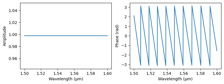
We can also plot the transmission:

import matplotlib.pyplot as plt

wls = jnp.linspace(1.5, 1.6, 1000)
transmission = waveguide_toy_model(wl=wls, length=100.0, loss_db_per_cm=1)
s21 = transmission[("o1", "o2")]

plt.figure(figsize=(9, 3))
plt.subplot(1, 2, 1)
plt.plot(wls, jnp.abs(s21)**2)
plt.xlabel("Wavelength (µm)")
plt.ylabel("Amplitude")
plt.subplot(1, 2, 2)
plt.plot(wls, jnp.angle(s21))
plt.xlabel("Wavelength (µm)")
plt.ylabel("Phase (rad)")
plt.show()