Dispersion: Symbolic Regression#
import matplotlib.pyplot as plt
import numpy as np
import xarray as xr


ds = xr.load_dataset("data/neff_te0_db.nc")
print(ds)
<xarray.Dataset> Size: 10kB
Dimensions:     (wavelength: 61, top_width: 20)
Coordinates:
  * wavelength  (wavelength) float64 488B 1.4 1.405 1.41 ... 1.69 1.695 1.7
  * top_width   (top_width) float64 160B 0.3 0.32 0.34 0.36 ... 0.64 0.66 0.68
Data variables:
    neff_te0    (top_width, wavelength) float64 10kB 2.036 2.027 ... 2.463 2.459
wavelengths = ds["wavelength"].values
top_widths = ds["top_width"].values
neff = ds["neff_te0"].values
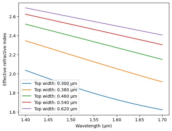
plt.figure()
plt.xlabel("Wavelength (µm)")
plt.ylabel("Effective refractive index")
for i in range(0, len(top_widths), 4):
plt.plot(wavelengths, neff[i], label=f"Top width: {top_widths[i]:.3f} µm")
plt.legend()
plt.show()
Symbolic Regression#
import numpy as np
from pysr import PySRRegressor
import xarray as xr
from itertools import product
from sklearn.preprocessing import StandardScaler
import matplotlib.pyplot as plt
from sklearn.metrics import r2_score, mean_squared_error
from matplotlib import pyplot as plt

ds = xr.load_dataset("data/neff_te0_db.nc")

coord_names = ["top_width", "wavelength"]
coords = [ds.coords[name].values for name in coord_names]

X = np.array(list(product(*coords)))
y = ds["neff_te0"].values.flatten()

# Normalize features
scaler_X = StandardScaler()
X_scaled = scaler_X.fit_transform(X)

scaler_y = StandardScaler()
y_scaled = scaler_y.fit_transform(y.reshape(-1, 1)).flatten()


model = PySRRegressor(
    niterations=400,
    populations=40,
    maxsize=40,
    verbosity=0
)
model.fit(X_scaled, y_scaled)
Detected IPython. Loading juliacall extension. See https://juliapy.github.io/PythonCall.jl/stable/compat/#IPython
/Users/vahid/doplaydo/doModels/.venv/lib/python3.12/site-packages/pysr/sr.py:2811: UserWarning: Note: it looks like you are running in Jupyter. The progress bar will be turned off.
  warnings.warn(
PySRRegressor.equations_ = [
	    pick         score                                           equation  \
	0         0.000000e+00                                                 x0
	1         3.201563e-02                                    x0 * 0.87595063
	2         5.158965e-01                            (x1 * -0.40640774) + x0
	3         1.026243e-01              (x0 * 0.87594867) - (x1 * 0.40640372)
	4         7.402805e-08  ((-1.6106493e-7 - x0) * -0.8759514) - (x1 * 0....
	5         7.478727e-01  ((x1 + ((x0 + -2.515248) * x0)) - 0.99999523) ...
	6         6.264657e-01  (((x1 * -0.41697693) + x0) + 0.27268115) * ((x...
	7         2.596142e-01  (((x0 * -0.2750113) + 1.593463) * (x0 + (2.609...
	8         4.555390e-01  (x0 - (((x0 * 0.07233008) - 0.40601394) * ((((...
	9         1.738736e-02  ((x0 * 1.1750462) - (((x0 * 0.0703593) - 0.406...
	10        2.600872e-01  ((-0.35148537 - (((x0 * (x0 * -0.67813367)) - ...
	11        1.533204e-03  ((-0.32173187 - ((((-0.72107697 * x0) * (x0 - ...
	12        7.522903e-02  ((-0.3548211 - (((((x0 * (x0 * (x1 * 0.0083031...
	13        1.416884e-01  ((-0.35471416 - (((x0 * (-0.11471766 + (x1 * (...
	14  >>>>  1.365409e-01  ((-0.31943703 - ((((x0 * -0.73160255) * (x0 - ...
	15        3.477136e-02  ((-0.61338526 - (((((((x0 * x1) * 0.014427088)...
	16        3.509060e-02  (((-0.8608156 - x0) - (((((((x0 * 0.020068347)...
	17        6.168531e-02  (((-0.871374 - x0) - ((((x0 * (x0 - -0.5435605...
	18        1.059197e-02  (((-0.86151135 - x0) - ((((((x0 + -0.19577916)...

	        loss  complexity
	0   0.248098           1
	1   0.232709           3
	2   0.082930           5
	3   0.067542           7
	4   0.067542           9
	5   0.015135          11
	6   0.004324          13
	7   0.002572          15
	8   0.000416          19
	9   0.000402          21
	10  0.000239          23
	11  0.000238          25
	12  0.000205          27
	13  0.000154          29
	14  0.000117          31
	15  0.000110          33
	16  0.000102          35
	17  0.000090          37
	18  0.000088          39
]
In a Jupyter environment, please rerun this cell to show the HTML representation or trust the notebook.
On GitHub, the HTML representation is unable to render, please try loading this page with nbviewer.org.
Parameters
| model_selection | 'best' | |
| binary_operators | None | |
| unary_operators | None | |
| expression_spec | None | |
| niterations | 400 | |
| populations | 40 | |
| population_size | 27 | |
| max_evals | None | |
| maxsize | 40 | |
| maxdepth | None | |
| warmup_maxsize_by | None | |
| timeout_in_seconds | None | |
| constraints | None | |
| nested_constraints | None | |
| elementwise_loss | None | |
| loss_function | None | |
| loss_function_expression | None | |
| loss_scale | 'log' | |
| complexity_of_operators | None | |
| complexity_of_constants | None | |
| complexity_of_variables | None | |
| complexity_mapping | None | |
| parsimony | 0.0 | |
| dimensional_constraint_penalty | None | |
| dimensionless_constants_only | False | |
| use_frequency | True | |
| use_frequency_in_tournament | True | |
| adaptive_parsimony_scaling | 1040.0 | |
| alpha | 3.17 | |
| annealing | False | |
| early_stop_condition | None | |
| ncycles_per_iteration | 380 | |
| fraction_replaced | 0.00036 | |
| fraction_replaced_hof | 0.0614 | |
| weight_add_node | 2.47 | |
| weight_insert_node | 0.0112 | |
| weight_delete_node | 0.87 | |
| weight_do_nothing | 0.273 | |
| weight_mutate_constant | 0.0346 | |
| weight_mutate_operator | 0.293 | |
| weight_swap_operands | 0.198 | |
| weight_rotate_tree | 4.26 | |
| weight_randomize | 0.000502 | |
| weight_simplify | 0.00209 | |
| weight_optimize | 0.0 | |
| crossover_probability | 0.0259 | |
| skip_mutation_failures | True | |
| migration | True | |
| hof_migration | True | |
| topn | 12 | |
| should_simplify | True | |
| should_optimize_constants | True | |
| optimizer_algorithm | 'BFGS' | |
| optimizer_nrestarts | 2 | |
| optimizer_f_calls_limit | None | |
| optimize_probability | 0.14 | |
| optimizer_iterations | 8 | |
| perturbation_factor | 0.129 | |
| probability_negate_constant | 0.00743 | |
| tournament_selection_n | 15 | |
| tournament_selection_p | 0.982 | |
| parallelism | None | |
| procs | None | |
| cluster_manager | None | |
| heap_size_hint_in_bytes | None | |
| batching | False | |
| batch_size | 50 | |
| fast_cycle | False | |
| turbo | False | |
| bumper | False | |
| precision | 32 | |
| autodiff_backend | None | |
| random_state | None | |
| deterministic | False | |
| warm_start | False | |
| verbosity | 0 | |
| update_verbosity | None | |
| print_precision | 5 | |
| progress | True | |
| logger_spec | None | |
| input_stream | 'stdin' | |
| run_id | None | |
| output_directory | None | |
| temp_equation_file | False | |
| tempdir | None | |
| delete_tempfiles | True | |
| update | False | |
| output_jax_format | False | |
| output_torch_format | False | |
| extra_sympy_mappings | None | |
| extra_torch_mappings | None | |
| extra_jax_mappings | None | |
| denoise | False | |
| select_k_features | None |
Show code cell source
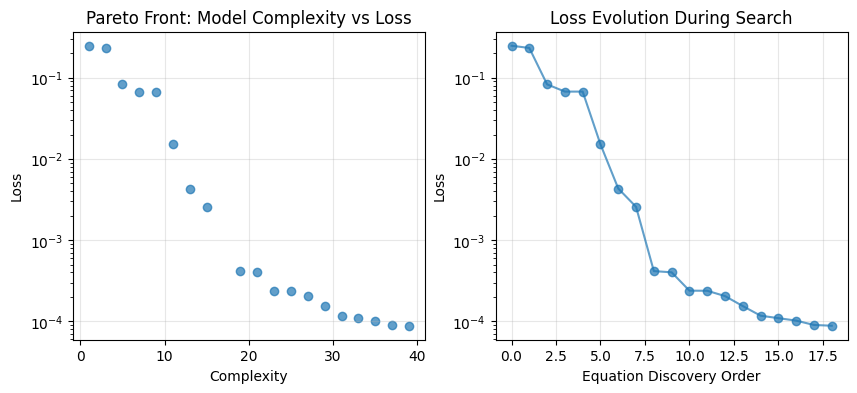
# Get all equations and their metrics
equations_df = model.equations_

# Plot complexity vs loss (Pareto front)
plt.figure(figsize=(10, 4))

plt.subplot(1,2,1)
plt.scatter(equations_df['complexity'], equations_df['loss'], alpha=0.7)
plt.xlabel('Complexity')
plt.ylabel('Loss')
plt.title('Pareto Front: Model Complexity vs Loss')
plt.yscale('log')  # Often helpful since loss can vary by orders of magnitude
plt.grid(True, alpha=0.3)

# Plot loss vs equation index (discovery order)
plt.subplot(1,2,2)
plt.plot(equations_df.index, equations_df['loss'], 'o-', alpha=0.7)
plt.xlabel('Equation Discovery Order')
plt.ylabel('Loss')
plt.title('Loss Evolution During Search')
plt.yscale('log')
plt.grid(True, alpha=0.3)
# For predictions, transform back
y_pred_scaled = model.predict(X_scaled)
y_pred = scaler_y.inverse_transform(y_pred_scaled.reshape(-1, 1)).flatten()
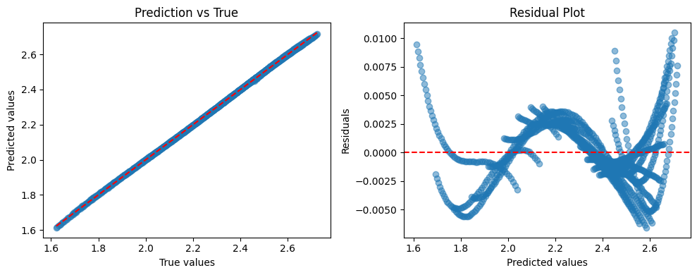
print(f"R² score: {r2_score(y, y_pred):.4f}")
print(f"RMSE: {np.sqrt(mean_squared_error(y, y_pred)):.4f}")
R² score: 0.9999
RMSE: 0.0028
Show code cell source
# Plot comparison
plt.figure(figsize=(10, 4))
plt.subplot(1, 2, 1)
plt.scatter(y, y_pred, alpha=0.5)
plt.plot([y.min(), y.max()], [y.min(), y.max()], "r--")
plt.xlabel("True values")
plt.ylabel("Predicted values")
plt.title("Prediction vs True")

plt.subplot(1, 2, 2)
residuals = y - y_pred
plt.scatter(y_pred, residuals, alpha=0.5)
plt.axhline(y=0, color="r", linestyle="--")
plt.xlabel("Predicted values")
plt.ylabel("Residuals")
plt.title("Residual Plot")

plt.tight_layout()
Show code cell source
import numpy as np
import matplotlib.pyplot as plt
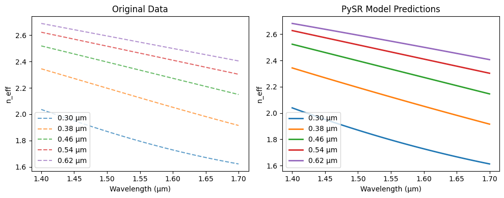
wavelengths = ds.wavelength.values
selected_top_widths = ds.top_width.values[::4]
plt.figure(figsize=(10, 4))
plt.subplot(1,2,1)
for tw in selected_top_widths:
if tw in ds.top_width.values: # Only plot if the exact value exists
plt.plot(ds.wavelength, ds.neff_te0.sel(top_width=tw),
label=f"{tw:.2f} µm", linestyle="--", alpha=0.7)
plt.xlabel("Wavelength (µm)")
plt.ylabel("n_eff")
plt.title("Original Data")
plt.legend()
plt.subplot(1,2,2)
for tw in selected_top_widths:
# Create input array for this top_width across all wavelengths
X_pred = np.column_stack([
np.full(len(wavelengths), tw), # constant top_width
wavelengths # varying wavelength
])
X_pred_scaled = scaler_X.transform(X_pred)
y_pred_scaled = model.predict(X_pred_scaled)
y_pred = scaler_y.inverse_transform(y_pred_scaled.reshape(-1, 1)).flatten()
plt.plot(wavelengths, y_pred, label=f"{tw:.2f} µm", linewidth=2)
plt.xlabel("Wavelength (µm)")
plt.ylabel("n_eff")
plt.title("PySR Model Predictions")
plt.legend()
plt.tight_layout()
Show code cell source
# from sympy import symbols
# a = model.sympy()
# a.subs([(symbols("x0"), symbols("w")),
#         (symbols("x1"), symbols("λ"))])
# # type(a)


# 1. Get the scaled symbolic expression
expr_scaled = model.sympy()

# 3. Apply inverse y-scaling
y_mean = scaler_y.mean_[0]
y_std = scaler_y.scale_[0]
expr_rescaled = y_std * expr_scaled + y_mean

model.sympy()
\[\displaystyle \left(- x_{0} - \left(x_{0} \left(x_{1} x_{0} \left(0.66593647 - x_{0}\right) \left(-0.007577593\right) - 0.10187686\right) - -0.47428933\right) \left(x_{0} \left(-0.73160255\right) \left(x_{0} - -0.30258545\right) - x_{1}\right) - 0.31943703\right) \left(-0.8628376\right)\]