CMT: Intro

In this chapter (as well as the next two chapters) we develop semi-analytical models based on coupled mode theory discussed in this paper: Design Space Exploration of Microring Resonators in Silicon Photonic Interconnects: Impact of the Ring Curvature

(Another good read for a simpler case is Evanescent waveguide couplers)

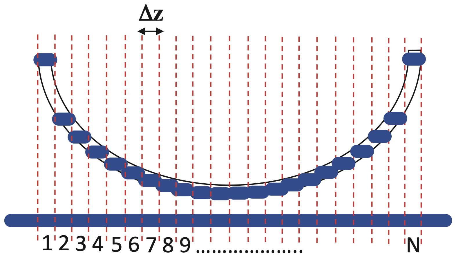
The main idea is to discretize the coupling area into many sections, each approximated as a simple directional coupler with a fixed gap:

Imports

```python import doModels.RefractiveIndex as ri import doModels.fem as fem import doModels.SemiAnalyticalCouplers as analyze

import matplotlib.pyplot as plt import numpy as np import xarray as xr from datetime import datetime from tqdm.notebook import tqdm ```

Define Stack

python stack = fem.CoupledWaveguides(gap=0.2, w_core_1=0.45, w_core_2=0.45, h_core=0.22, n_clad_func=ri.silica, n_core_func=ri.silicon)

Database of Coupled Waveguides

First, we create a database of super-modes for two adjacent waveguides whilst sweeping gap and wavelength. We use FEMWELL as described in Chapter 5. We store the results in an xarray netcdf file.

```python num_modes = 2 _gap = np.linspace(0.1, 0.9, 25) _wavelength = np.arange(1.5, 1.6, 0.005)

n = np.zeros((num_modes, len(_gap), len(_wavelength)))

for i, gap in enumerate(tqdm(_gap)): for j, wavelength in enumerate(_wavelength): stack.gap = gap modes = fem.supermode_solver( coupled_waveguides=stack, wavelength=wavelength, num_modes=num_modes, resolution=0.02, ) n[:, i, j] = modes

ds = xr.Dataset( { f"n{k+1}": (["gap", "wavelength"], n[k, :, :]) for k in range(num_modes) }, coords={"gap": _gap, "wavelength": _wavelength}, )

ds_sorted = analyze.adiabatic_mode_tracker1(ds) ds_sorted.to_netcdf("data/coupled_wgs.nc")

print(ds) ```

Load Database

python ds = xr.load_dataset("data/coupled_wgs.nc") analyze.plot_interpolated_modes(ds, wl=1.55, gap=0.3)

Exponential Fit

In the paper we cited above, the authors make a few geometrical arguments and apply some approximations to come up with a closed form expression for coupling coefficients of the directional coupler (See Eq. 11). One is to assume the indices of these supermodes follow an exponential as a function of gap:

```python aE, gammaE, aO, gammaO = analyze.fit_supermodes(ds, interp_at={"wavelength":1.55}, plot=True)

```

Compute Coupling Coefficient

Following Eq. 11, we compute the coupling coefficient \(\kappa\) as a function of gap, wavelength, and length.

```python

--- Plot κ vs gap ---

lambda_µm = 1.55 gaps_µm = np.linspace(0.250, 0.9, 100) lengths_µm = [1, 10, 50] kappa_results = np.zeros((len(lengths_µm), len(gaps_µm)))

fit_params = {} fit_params['aE'], fit_params['gammaE'], fit_params['aO'], fit_params['gammaO'] = analyze.fit_supermodes(ds, interp_at={"wavelength":lambda_µm})

for i, length_x_µm in enumerate(lengths_µm): for j, d in enumerate(gaps_µm): kappa_results[i, j] = analyze.kappa_directional_coupler(gap_µm=d, R_µm=20, lambda_µm=lambda_µm, length_x_µm=length_x_µm, v_offset_µm=15, fit_params=fit_params, wg_width_µm=stack.w_core_1)

plt.figure() for i, length_x_µm in enumerate(lengths_µm): plt.plot(gaps_µm, kappa_results[i], label=f'l_x = {length_x_µm} µm') plt.xlabel('Gap (µm)') plt.ylabel('κ') plt.grid(True) plt.legend()

--- Plot κ vs wavelength for fixed gaps ---

wavelengths_µm = np.linspace(1.50, 1.599, 100) fixed_gaps = [0.3, 0.4, 0.5]

plt.figure() for d in fixed_gaps: kappa_vals = [] for λ in wavelengths_µm: params = analyze.fit_supermodes(ds, interp_at={"wavelength": λ}, plot=False) kappa = analyze.kappa_directional_coupler(gap_µm=d, R_µm=20, lambda_µm=λ, length_x_µm=10, # or any fixed length v_offset_µm=15, fit_params=dict(zip(['aE', 'gammaE', 'aO', 'gammaO'], params)), wg_width_µm=stack.w_core_1) kappa_vals.append(kappa) plt.plot(wavelengths_µm, kappa_vals, label=f'gap = {d} µm')

plt.xlabel('Wavelength (µm)') plt.ylabel('κ') plt.grid(True) plt.legend() ```

To better visualize the coupling coefficient, we precomputed it for a range of parameters (gap, radius, length_x, and v_offset, wavelength) and store them in a look-up table. This is the simplest way to create an interactive plot shown in the next page.

```python

Define ranges

gap_vals = np.arange(0.25, 0.9, 0.04) # gaps in µm radius_vals = np.arange(5, 100, 20) # radii in µm wavelengths = np.arange(1.5, 1.6 , 0.005) # wavelengths in µm length_x_vals = np.arange(0, 100, 8) v_offset_vals = np.arange(5, 100, 40)

Initialize array

kappa_array = np.zeros((len(wavelengths), len(gap_vals), len(radius_vals), len(length_x_vals), len(v_offset_vals)))

for i0, wl in enumerate(wavelengths): fit_params = {} fit_params['aE'], fit_params['gammaE'], fit_params['aO'], fit_params['gammaO'] = analyze.fit_supermodes(ds_sorted, interp_at={"wavelength":wl})

for i1, gap in enumerate(gap_vals):
    for i2, radius in enumerate(radius_vals):
        for i3, length_x in enumerate(length_x_vals):
            for i4, v_offset in enumerate(v_offset_vals):
                kappa_array[i0, i1, i2, i3, i4] = analyze.kappa_directional_coupler(gap_µm=gap, 
                                        R_µm=radius, 
                                        lambda_µm=wl, 
                                        length_x_µm=length_x, 
                                        v_offset_µm=v_offset, 
                                        fit_params=fit_params, 
                                        wg_width_µm=stack.w_core_1)
                if np.isnan(kappa_array[i0, i1, i2, i3, i4]):
                    print(gap, radius, wl, length_x)

xarr_out = xr.DataArray( data=kappa_array, coords={ "wavelength": wavelengths, "gap": gap_vals, "radius": radius_vals, "length_x": length_x_vals, "v_offset": v_offset_vals, }, dims=["wavelength", "gap", "radius", "length_x", "v_offset"], name="kappa" )

xarr_out.to_netcdf("data/directional_coupler.nc")

xarr_out.to_dataframe().reset_index().to_json("data/directional_coupler.json", orient="records") ```